Classifier-Free Guidance: The Guidance Scale Is an Exponent on an Implicit Classifier

Classifier-free guidance (CFG) trains a conditional generative model with condition dropout, so one network can predict both with and without the conditioning signal. At sampling time the two predictions are combined by extrapolating along their difference, scaled by a guidance weight. Nearly every modern conditional generator exposes that weight: image diffusion models, the per-token diffusion heads that autoregressive TTS systems run on top of an LLM backbone, and, per decoding step, token language models.
The scale is widely described as conditioning strength. That framing predicts the benefit, stronger adherence to the condition, and none of the costs. By Bayes rule, the difference between the conditional and unconditional predictions estimates the gradient of a classifier the generative model already contains, and the guidance weight is an exponent on that classifier's probability. That one fact is what makes the rest predictable: CFG sharpens the sampling distribution rather than improving the model, costs a second forward pass per step, trades diversity for per-sample fidelity, pushes the sampler off its training distribution at high scales, and has no portable "good value", because the exponent multiplies a quantity whose magnitude is system-specific.
Classifier guidance needed a separate noise-aware classifier
CFG replaced an earlier construction. A diffusion model's denoising network eps(x_t, c) predicts the noise mixed into the current iterate x_t, and up to a known negative scale factor that prediction estimates the score, the gradient of the log density of the noised data. Bayes rule splits the conditional score into two terms:
grad log p_t(x | c) = grad log p_t(x) + grad log p_t(c | x)
Dhariwal and Nichol exploited the second term directly: train a separate classifier p(c | x_t) and add its input-gradient, multiplied by a scale s, to the diffusion model's score at every sampling step. The classifier must be trained on noised inputs at every noise level the sampler visits, because a clean-data classifier produces meaningless gradients on the noisy iterates the sampler actually queries.
The scale was already an exponent there. Multiplying the gradient by s turns p(c | x) into p(c | x)^s inside the log, and as a function of x that term up-weights the inputs the classifier assigns to c most confidently, more aggressively as s grows. The exponent was not optional. Guiding an unconditional ImageNet model at s = 1, which is exactly the Bayes decomposition, produced samples that did not visibly match their classes even though the classifier scored them near 50%: the estimated gradient is too weak in practice to carry the conditioning alone. Pushing s from 1 to 10 on ImageNet traded recall (a coverage measure of diversity) from 0.52 down to 0.32 while precision rose from 0.82 to 0.88. The construction worked but carried an operational burden: a separate noise-aware classifier per conditioning type, and for a condition richer than a class label, a free-text prompt, there is no off-the-shelf classifier to train.
Bayes rule removes the classifier network, not the classification
Ho and Salimans inverted the same identity. The implicit classifier inside any conditional generative model is p(c | x) proportional to p(x | c) / p(x), so its gradient is the difference between the conditional and unconditional scores. A diffusion model that can produce both predictions does not need the external classifier; the subtraction eps(x_t, c) minus eps(x_t) plays its role.
Both predictions come from one network. During training the condition c is replaced with probability p_uncond by a null token, a learned embedding standing for "no condition", so the same weights learn p(x | c) and p(x) jointly. In their ablation, dropout rates of 0.1 and 0.2 perform about equally and 0.5 is consistently worse: the unconditional branch needs only a minority of training capacity. Sampling combines the two outputs:
eps_guided = (1 + w) * eps(x_t, c) - w * eps(x_t)
with guidance strength w, where w = 0 is plain conditional sampling. Most codebases reparameterize with s = 1 + w:
eps_guided = eps_uncond + s * (eps_cond - eps_uncond)
so s = 1 means guidance off. The two conventions differ by exactly one, both are in active use, and published "guidance scale" numbers are not comparable without the accompanying equation.
The cost is structural: every sampling step evaluates the full network twice, once per branch, usually run as a doubled batch. When that matters, the guided pair can be distilled into a single student network that matches the combined output directly (Meng et al. 2022), moving the cost from every deployment step to a one-time training job.
The scale tilts the sampling distribution toward the implicit classifier's modes
Substituting the implicit classifier back into the classifier-guidance formula shows what the sampler is being pointed at, per noise level:
grad log [ p_t(x | c) * p_implicit(c | x)^w ]
Each denoising step moves toward a tilted distribution: the model's own conditional, multiplied by the implicit classifier raised to the guidance power. Geometrically, the update extrapolates past the conditional prediction, directly away from the unconditional one: away from what the model expects regardless of the condition, deeper into the region that only the condition explains.
Two gaps separate that picture from exact sampling, and Ho and Salimans state the first themselves: the epsilon outputs are unconstrained network outputs, so their difference is not in general the gradient of any actual classifier. The second is that even with exact scores, steering each noise level toward its tilted marginal does not compose into sampling the tilted data distribution; Bradley and Nakkiran later showed that CFG instead matches a predictor-corrector sampler, alternating a denoising step with a sharpening correction. CFG is a per-step correction that reliably lands in high-confidence regions of the implicit classifier, not exact inference over a known distribution.
The exponent reading predicts the measured trade-offs. Concentrating mass on classifier modes should hurt distribution-level metrics first and per-sample metrics last, and it does: on ImageNet 64x64, FID (a distribution distance that punishes diversity loss and per-sample artifacts alike) is best at the barely-on w = 0.1 and degrades about seventeenfold by w = 4, while Inception Score, which rewards confidently recognizable individual samples, rises monotonically over the same sweep. Ho and Salimans describe the visual version plainly: sample variety decreases as individual sample fidelity increases.
Pushed further, guidance breaks the sampler's own input distribution. The Imagen authors traced high-guidance failure to a train-test mismatch: the guided update implies clean-image estimates outside the [-1, 1] range of training images, the sampler iterates on its own out-of-range outputs, and images come out saturated and unnatural or diverge outright. Their fix, dynamic thresholding, re-clamps the implied clean-image estimate at every step. The portable lesson is the mechanism, not the fix: extrapolation queries the network off its training manifold, and what breaks first is whatever your domain's analog of pixel range is.
The same extrapolation runs per token on logits in autoregressive models
Nothing in the construction is diffusion-specific; it needs only two predictions from one network that differ in conditioning. In discrete autoregressive models the combination runs once per decoding step, on logits. Koel-TTS, an encoder-decoder TTS token model, trains with both the text and the reference speaker audio dropped together at probability 0.1, then decodes with
logits_guided = logits_uncond + gamma * (logits_cond - logits_uncond)
before the softmax, where gamma sits in the s-convention (gamma = 1 is guidance off). Here the tilt is exact where diffusion's is heuristic: the softmax renormalizes, so each token is sampled from precisely p_cond^gamma times p_uncond^(1-gamma), normalized. The exactness is per token: the product of per-token tilts is not the tilted distribution over whole sequences, where the same caveat reappears one level up. The unconditional branch consumes the same generated token history with no text or speaker prefix, so its prediction answers "how would this audio continue with no instructions", and the guided difference amplifies exactly what the instructions explain. Text LLMs use the same per-step recipe to amplify a prompt, contrasting predictions with and without it (Sanchez et al. 2023), and the two branches' different prefixes mean AR CFG doubles the KV cache as well as the per-token compute.
The trade-off lands differently in TTS than in images. Sweeping gamma from 1 to 3, Koel-TTS finds character error rate and speaker-embedding similarity improve together, with the optimum at 2.5: both metrics measure adherence to a conditioning input being amplified, and much of the "diversity" being burned is the unconditioned failure mode, hallucinated words and drifting voice. The cost surfaces where the paper notes it, as reduced variation at higher scales, not in the adherence metrics.
The unconditional branch defines what you extrapolate away from
What the second branch conditions on is a design choice, and systems diverge on it. Koel-TTS drops text and speaker context together, so guidance amplifies both at once. VibeVoice's report describes no trained null token: its diffusion head's unconditional branch conditions on the hidden state of the start-of-sequence token, a minimally conditioned input the model computes anyway. SemaVoice drops the LLM hidden state but keeps the previously generated acoustic patch in the unconditional branch, so patch-to-patch continuity stays unguided and only the semantic conditioning is sharpened. The negative-prompt field in image generators is this same equation with the null condition replaced by an unwanted description, turning "away from what is typical" into "away from what is specified".
Two refinements push the lever further. InstructPix2Pix decomposes the condition and runs two differences with two scales, one amplifying agreement with the input image and one with the edit instruction, the practical alternative to dropping all conditions jointly the way Koel-TTS does. Autoguidance (Karras et al. 2024) replaces the unconditional branch with a smaller, less-trained version of the same model, so the extrapolation points away from that weaker model's errors rather than away from the condition's absence, and recovers fidelity without the diversity collapse. In every case the guided sample is defined as much by the negative branch as by the positive one.
Tuned scales do not transfer across systems, tasks, or notation conventions
Speech systems that all cite the same CFG paper (we locate these architectures in our map of the modern speech stack) ship guidance settings spanning a factor of three, at different denoising step counts:
| System | CFG site | Published setting | In s-convention (s = 1 is off) | Head denoising steps |
|---|---|---|---|---|
| VibeVoice | per-token diffusion head | 1.3 | 1.3 | 10 |
| Koel-TTS | AR token logits | gamma = 2.5 | 2.5 | none (token model) |
| SemaVoice | per-patch diffusion head | w = 2.5 | 3.5 | not stated |
| LatentLM (TTS) | per-token diffusion head | 4 | 4 | 5 |
| LatentLM (ImageNet) | per-token diffusion head | 1.65 | 1.65 | not stated |
Source: VibeVoice Sec. 3.2 and Fig. 3; Koel-TTS Secs. 2.5 and 3.4; SemaVoice Sec. 3.2.3 (which uses the (1+w) convention, hence the conversion); LatentLM Secs. 3.1 and 3.3.6.
LatentLM is one architecture family, and it needs 1.65 for class-conditional ImageNet but 4 for TTS: neither the architecture nor the codebase pins the value, the task does. And SemaVoice's published 2.5 is 3.5 in the convention the other rows use, because its paper writes the Ho-Salimans (1+w) form; copying a guidance number without its equation silently changes the strength by one full unit.
The spread follows from the exponent reading: the scale multiplies the implicit classifier's log-likelihood ratio, and the magnitude of that ratio depends on how strongly the conditioning pins the output (a transcript plus a speaker prompt constrains speech far harder than a class label constrains an image), on what the unconditional branch conditions on, and on the sampler's step count. The guidance scale is a coefficient on a system-specific signal, not an absolute strength in shared units.
Published sweeps differ in shape, not just in optimum:
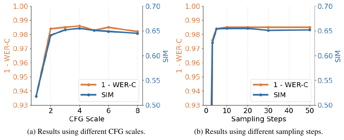
LatentLM paper, Figure 10, p. 14: intelligibility (1 - WER-C, where WER-C is word error rate from a Conformer-Transducer ASR transcription) and speaker similarity over CFG scales 1 to 8 and over diffusion sampling steps. The jump from scale 1 (guidance off) to 2 dwarfs everything after it, and the optimum at 4 sits on a broad plateau.
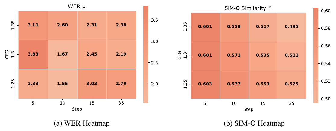
VibeVoice paper, Figure 3, p. 8: word error rate and SIM-O (speaker-embedding similarity to the reference audio) over CFG scales 1.25 to 1.35 and denoising steps 5 to 35. Within that narrow scale window, WER still swings from 3.83 to 1.55 depending on the scale-step pair, and the WER optimum (scale 1.25 at 10 steps) disagrees with the similarity optimum (5 steps), so the shipped setting of 1.3 at 10 steps is a compromise.
The operational consequence: treat the guidance scale and step count as one jointly swept pair per system, and when reporting the result, publish the combination equation next to the number. A scale without its equation is not a reproducible setting.
Sources
- Ho & Salimans, Classifier-Free Diffusion Guidance (arXiv 2207.12598): condition-dropout training and p_uncond ablation (Table 1), the guided combination and w convention (Eq. 6), the implicit-classifier derivation and the not-a-real-gradient caveat, the two-evaluation cost, and the ImageNet 64x64 FID/IS sweep.
- Dhariwal & Nichol, Diffusion Models Beat GANs on Image Synthesis (arXiv 2105.05233): classifier guidance mechanics, noise-aware classifier requirement, gradient scaling as the exponent on p(c|x), the s = 1 failure on an unconditional model, and the precision/recall trade (Table 4).
- Saharia et al., Imagen (arXiv 2205.11487): high-guidance train-test mismatch, out-of-range clean-image estimates, saturation, and dynamic thresholding.
- Bradley & Nakkiran, Classifier-Free Guidance is a Predictor-Corrector (arXiv 2408.09000): CFG does not sample the tilted distribution; supports the exact-sampling caveat.
- Koel-TTS (arXiv 2502.05236): logit-space CFG for an AR TTS model (Sec. 2.5), 10% joint dropout, the gamma sweep and optimum (Sec. 3.4, Fig. 4), and the doubled effective batch.
- LatentLM, Multimodal Latent Language Modeling with Next-Token Diffusion (arXiv 2412.08635): TTS CFG and step ablations (Fig. 10), image-generation guidance settings (Sec. 3.1), WER-C metric definition (Sec. 3.3).
- VibeVoice (OpenReview, ICLR 2026): diffusion-head CFG with the start-of-sequence unconditional branch (Eq. 6), shipped settings (Sec. 3.2), and the scale-step heatmaps (Fig. 3). The shorter arXiv technical report (2508.19205) omits the heatmap figure.
- SemaVoice (arXiv 2605.16964): LLM-state dropout with retained previous patch, (1+w) convention at w = 2.5 (Sec. 3.2.3).
- Sanchez et al., Stay on Topic with Classifier-Free Guidance (arXiv 2306.17806): per-step logit CFG in pure text LLMs.
- Brooks et al., InstructPix2Pix (arXiv 2211.09800): two-condition CFG with independent guidance scales (Eq. 3).
- Karras et al., Guiding a Diffusion Model with a Bad Version of Itself (arXiv 2406.02507): autoguidance; replacing the unconditional branch with a degraded model.
- Meng et al., On Distillation of Guided Diffusion Models (arXiv 2210.03142): removing the two-pass cost by distilling the guided pair.