Flow Matching: Regress the Field the Sampler Integrates
Flow matching trains a continuous normalizing flow: a generative model that parameterizes a time-dependent vector field v_theta(x, t) with a neural network and produces samples by drawing noise x_0 from N(0, I) and integrating the ODE dx/dt = v_theta(x, t) from t = 0 to t = 1. The training objective, introduced by Lipman et al., is plain least squares: choose a probability path p_t that interpolates between the noise distribution and the data distribution, and regress v_theta onto the velocity field u_t that generates that path, meaning that transporting samples along u_t reproduces p_t at every t.
L_FM = E_{t, x ~ p_t} || v_theta(x, t) - u_t(x) ||^2
Two properties make this the default way to train continuous generators. The regression target is the same field the ODE solver integrates at sampling time, and its scale can be made uniform over t, which together make training markedly more robust than score matching at identical architecture and compute. And the path is a free choice rather than the byproduct of a diffusion process, which admits the straight optimal-transport path: a velocity target that is constant in time during training, and, empirically, the same sample quality at a fraction of the solver steps.
Per-example velocity targets optimize the intractable marginal objective
The loss above cannot be computed as written: for any path that ends at the data distribution, u_t depends on the unknown data density, so there is nothing to regress onto. Conditional flow matching (CFM) is the construction that fixes this. Condition on one data sample x_1 and define a per-example Gaussian path p_t(x | x_1) that starts at standard noise at t = 0 and ends at a concentrated Gaussian N(x_1, sigma_min^2 I) around the sample at t = 1, with sigma_min a small constant, typically 1e-5. Marginalizing over the data distribution q(x_1) yields a path whose endpoint approximates the data. Writing x_t for a sample on the path at time t, the field that generates this marginal path is the average of the conditional fields over every x_1 that could have produced the observed x_t, weighted by the posterior:
u_t(x) = E[ u_t(x | x_1) | x_t = x ]
The CFM loss regresses the network onto the per-example targets instead:
L_CFM = E_{t, x_1 ~ q, x ~ p_t(x | x_1)} || v_theta(x, t) - u_t(x | x_1) ||^2
This works because of what least squares does with targets that vary given the input: the minimizing function is their conditional expectation, which by the equation above is exactly the marginal field. Lipman et al. prove the two statements that make this exact: the marginal field assembled from conditional fields generates the marginal path (Theorem 1), and L_CFM and L_FM differ by a constant independent of theta, so their gradients are identical (Theorem 2). Training on closed-form per-example targets therefore optimizes the intractable marginal objective exactly, in expectation. The construction is the same one denoising score matching uses for diffusion models, generalized from scores to arbitrary velocity fields.
For a Gaussian conditional path N(mu_t(x_1), sigma_t(x_1)^2 I), the affine map psi_t(x) = sigma_t(x_1) x + mu_t(x_1) pushes standard noise onto the path, and Theorem 3 derives the unique field whose flow is that map (primes denote time derivatives):
u_t(x | x_1) = (sigma_t'(x_1) / sigma_t(x_1)) (x - mu_t(x_1)) + mu_t'(x_1)
A training step is then: sample t uniformly on [0, 1], a data sample x_1, and noise x_0; form x_t = sigma_t(x_1) x_0 + mu_t(x_1); take a gradient step on the squared error against the closed-form target. No ODE is solved during training. Papers do not share a time convention (the flow-matching paper puts noise at t = 0 and data at t = 1; much of the diffusion literature and several flow-matching systems run the other way), and velocity signs flip with the convention, so equations cannot be copied across papers without checking it.
The path is a free choice: diffusion paths are special cases, the OT path is the alternative
The other half of the framework is that mu_t and sigma_t are free choices. Setting them to the schedule of the variance-preserving (VP) diffusion process recovers that diffusion path exactly, and the conditional field Theorem 3 assigns it coincides with the drift of score-based diffusion's probability-flow ODE (Appendix D of the paper). Deterministic diffusion sampling and flow-matching sampling are therefore the same operation, an ODE solve, and on the same path the ideal field is identical. What distinguishes the methods is the regressed quantity, its loss weighting, and which paths the construction can express: diffusion paths must arise from a forward noising process, and one inherited consequence is that they never reach the noise distribution in finite time, so the prior at t = 0 is only ever approximated.
The optimal-transport (OT) path makes mean and standard deviation linear in time:
mu_t(x_1) = t x_1          sigma_t(x_1) = 1 - (1 - sigma_min) t
x_t = (1 - (1 - sigma_min) t) x_0 + t x_1
u_t(x_t | x_1) = x_1 - (1 - sigma_min) x_0
The conditional flow is the optimal-transport displacement map between the two endpoint Gaussians: each conditional sample moves along a straight line at constant speed, the minimal-cost interpolation under squared distance. Along its own trajectory, the regression target is the constant x_1 - (1 - sigma_min) x_0; as a field over all of space, u_t factors as g(t) h(x | x_1), so its direction at any point never changes and only its scale depends on t, a simpler regression target than one that rotates as t advances. And conditional sampling trajectories stay straight, where diffusion-path trajectories can overshoot the endpoint and backtrack.
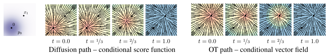
Source: Flow Matching for Generative Modeling, Figure 2, p. 6. What to see: across the four time panels, the diffusion path's conditional score (left) changes direction and magnitude as t advances, while the OT path's conditional vector field (right) keeps a constant direction.
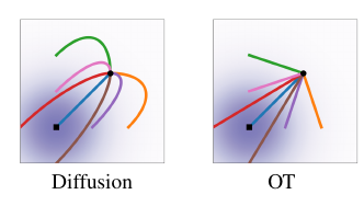
Source: Flow Matching for Generative Modeling, Figure 3, p. 6. What to see: trajectories of the diffusion conditional field (left) curve and backtrack; the OT conditional trajectories (right) run straight to the same endpoints.
Conditional optimality does not make the marginal flow an optimal-transport map. Where conditional paths cross, the marginal field is a posterior average of disagreeing conditional velocities, so marginal trajectories still curve; the paper claims only that the marginal field stays relatively simple, and closing this gap is what rectified flow's reflow procedure and minibatch OT coupling target.
The score target's scale diverges; the velocity loss measures the field the solver integrates
Two mechanisms separate the objectives. The first is target scale. For a Gaussian conditional path, the score (the gradient of the log density, which diffusion training regresses onto) is -(x - mu_t) / sigma_t^2 = -x_0 / sigma_t, with expected squared norm d / sigma_t^2 in d dimensions. As the path concentrates onto the data (sigma_t toward 0), the target's scale diverges, so an unweighted score regression is dominated by the times nearest the data, and every score-matching recipe inserts a per-time loss weight lambda(t) to compensate. The weightings are heuristics: Grad-TTS, a score-based TTS model, weights its per-time losses by lambda_t and states the rule it follows, that weights should be proportional to 1 / E||target||^2. The OT velocity target needs no weighting; its distribution is the same at every t. The same arithmetic says why a path ending in a near-point mass is trainable under velocity regression and pathological as a score target, whose norm at the endpoint scales as 1 / sigma_min.
The second is what the loss measures. The CFM loss is the squared error of the field the ODE solver will integrate, weighted uniformly over t. Score matching trains a score network, and the sampler then assembles the drift from it, with the score entering scaled by beta(1-t) / 2 on the VP path (beta is the VP noise schedule; the 1-t argument is the time-convention flip noted above). Converting squared score error into squared drift error therefore means weighting by (beta(1-t) / 2)^2, and neither standard recipe uses that weight: original score matching takes lambda(t) = sigma_t^2 and ScoreFlow takes beta(1-t). The trained loss and the error the solver accumulates are different time-weightings of the same error, so one can be low while the other is not.
Grad-TTS documents what that looks like: its diffusion loss converges early and then barely moves while output quality keeps improving across 1.7 million training iterations, and the authors' explanation is that score estimates inaccurate on a small subset of t barely move the weighted loss but break the ODE solve whenever the solver lands there. That much is true of any time-integrated loss, flow matching's included; what flow matching removes is the systematic mismatch. With an adaptive solver, the number of function evaluations (NFE, how many times the solver calls the network) needed to sample a score-matching model changes drastically over training, while the flow-matching models' sampling cost stays near its final value from the first epochs.
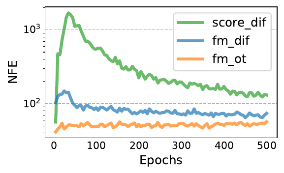
Source: Flow Matching for Generative Modeling, Figure 10, p. 21 (CIFAR-10, dopri5 solver at tolerance 1e-5). What to see: the score-matching curve (green) is the unstable one, spiking past 1,000 evaluations and drifting for hundreds of epochs, while both flow-matching curves stay near their final cost, the OT model (orange) cheapest.
Two ablations separate the objective from the path
The flow-matching paper trains the same U-Net architecture with the same hyperparameters under five configurations (three diffusion losses, flow matching on two paths), with the baselines allowed more training iterations to converge.
| Loss | ImageNet-64 FID | ImageNet-64 NFE | CIFAR-10 FID |
|---|---|---|---|
| DDPM (noise matching) | 17.36 | 264 | 7.48 |
| Score matching | 19.74 | 441 | 19.94 |
| ScoreFlow | 24.95 | 601 | 20.78 |
| FM, diffusion path | 16.88 | 187 | 8.06 |
| FM, OT path | 14.45 | 138 | 6.35 |
Source: Flow Matching for Generative Modeling, Table 1, p. 8. FID is Frechet Inception Distance, lower is better; the NFE column is the adaptive solver's evaluation count averaged over 50K samples. DDPM regresses the added noise; ScoreFlow is score matching with a likelihood-motivated weighting. None of these unconditional models is tuned for absolute state of the art (the paper suggests the architecture was not optimized for CIFAR-10 at all), so read the columns as controlled within-table contrasts.
FM with the OT path is best on every dataset and metric in the paper's full Table 1, test likelihood included. The within-path contrast carries the objective claim: holding the VP diffusion path fixed, the two score parameterizations degrade sharply on CIFAR-10 while the two constant-scale regression targets, DDPM's noise (a standard Gaussian at every t) and FM's velocity, stay stable. A well-conditioned target buys the stability whether it is noise or velocity; what noise matching does not buy is cheap integration, a roughly 40% higher adaptive-solver cost than FM on the identical path. The objective's advantage is robustness rather than uniform dominance: score matching edges FM-on-diffusion on ImageNet-32 (FID 5.68 against 6.37, with a lower adaptive NFE as well). Training cost moves the same direction, though only across papers: the ImageNet-128 FM-OT model reached its reported FID on a third fewer total training images than the ADM baseline of Dhariwal and Nichol, with a model 25% larger and otherwise differently tuned.
Voicebox replicates the factorization in speech: one model, one dataset, trained three ways (FM with the OT path, FM with the VP diffusion path, score matching with the same diffusion path), evaluated as zero-shot TTS by WER, the word error rate of an ASR model transcribing the synthesized speech. The comparison runs in a reduced setup with a lowered learning rate so that all three objectives converge.
| Objective | WER, 50K updates (NFE 32) | WER, 150K updates (NFE 32) | WER, 150K updates (NFE 4) |
|---|---|---|---|
| FM, OT path | 2.5 | 2.1 | 2.4 |
| FM, diffusion path | 76.0 | 2.6 | 11.5 |
| SM, diffusion path | 73.3 | 5.1 | 94.5 |
Source: Voicebox, the objective-comparison tables in Section 5.8 (Tables 8 and 9 in the arXiv version). For scale, ground-truth recordings score WER 2.2 on this evaluation.
At a 50K-update budget only the OT path yields a usable model; both diffusion-path variants still fail to produce intelligible speech. At 150K updates the objective swap on the identical path cuts WER roughly in half, and the path swap closes the rest of the gap to ground truth. In the low-NFE column both factors matter, but only the OT model stays usable at four evaluations, and score matching is still degraded at the table's maximum of 32.

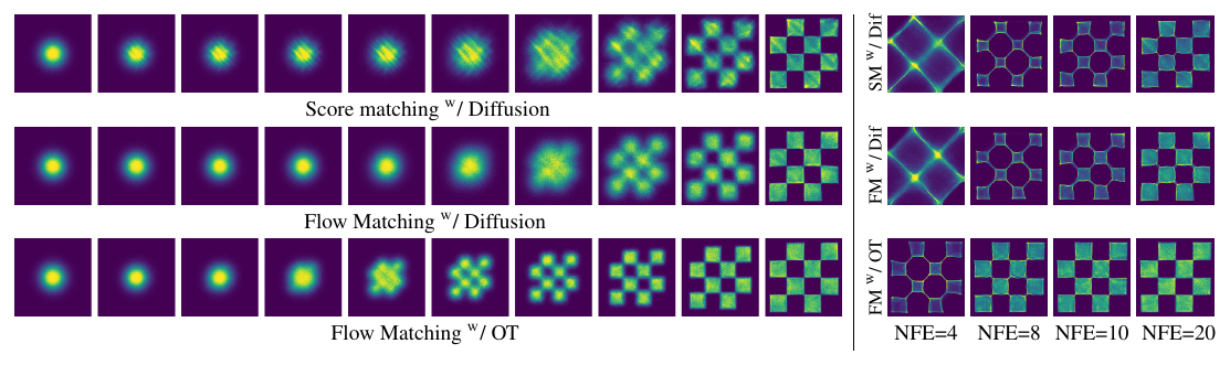
Source: Flow Matching for Generative Modeling, Figure 4, p. 7. What to see: on the left, the 2D checkerboard pattern emerges much earlier along the flow for FM with OT (bottom row) than for the diffusion-path models above it; on the right, FM-OT samples remain clean at NFE 4 to 20 while the other objectives' samples degrade.
Sampling: the NFE is chosen at inference time, and the path shifts the quality/NFE trade-off
Any off-the-shelf ODE solver turns a noise draw into a sample by integrating the learned field, and with a fixed-step solver the NFE is proportional to the step count, so the quality/latency operating point is chosen at inference time, per run, with no retraining. Deterministic diffusion samplers share that property; what the path changes is where the trade-off sits. On ImageNet-32 with the same fixed-step solvers, the FM-OT model reaches the same numerical error as the diffusion-path models with roughly 60% of the function evaluations and keeps usable FID at very low NFE, and Voicebox's NFE=4 column above is the speech version of the same gap.
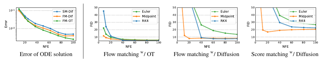
Source: Flow Matching for Generative Modeling, Figure 7, p. 9 (ImageNet-32, fixed-step solvers). What to see: in the left panel the FM-OT model (green) reaches a given numerical error at the fewest evaluations, and in the FID panels FM-OT sits near its converged quality at NFEs where score matching has not yet left the high-FID regime.
Classifier-free guidance transfers unchanged: train with condition dropout, then mix the conditional and unconditional fields at every solver step, which doubles the network evaluations for a fixed NFE. The mechanism, a guidance scale acting as an exponent on an implicit classifier, is covered in Classifier-Free Guidance: The Guidance Scale Is an Exponent on an Implicit Classifier. In audio the objective appears at more than one interface: Voicebox generates whole mel-spectrogram sequences with it, and a growing family generates the latents of a pretrained audio autoencoder, the setting whose encoder-side requirements are covered in Latent Audio Encoders: Reconstruction Sets the Ceiling, Not the Ranking. The objective also appears inside autoencoder training itself: SAME Makes Generation Difficulty an Autoencoder Training Loss trains a small flow-matching model jointly with a music autoencoder and backpropagates its loss into the encoder, shaping the latent space the downstream generator inherits.
Sources
- Lipman et al., Flow Matching for Generative Modeling (arXiv:2210.02747): FM and CFM objectives with Theorems 1-3, Sections 2-4 (objective section); Gaussian path family, VP and OT instances, and Figures 2 and 3, Section 4.1 (path section, both figures reproduced); probability-flow coincidence, Appendix D, and the score/noise-matching loss definitions with their weightings and the sampling drift, Appendix E (path and training-gap sections); Table 1, Figure 4, Figure 10, and the ImageNet-128 training budget, Section 6.1 (ablation section; Figure 4 reproduced as header and body figure, Figure 10 reproduced); the 60% NFE result and Figure 7, Section 6.2 (sampling section, figure reproduced).
- Le et al., Voicebox: Text-Guided Multilingual Universal Speech Generation at Scale (arXiv:2306.15687): flow matching with the OT path and classifier-free guidance for vector fields, Sections 3.1-3.5; the objective and path ablations, Section 5.8, Tables 8 and 9, with the reduced training setup in Appendix B.1 and the full grid in Table B4 (ablation and sampling sections); the ground-truth WER reference point in the English zero-shot TTS results table of Section 5.1.
- Popov et al., Grad-TTS: A Diffusion Probabilistic Model for Text-to-Speech (arXiv:2105.06337): the score-matching loss and its lambda_t weighting with the stated weighting heuristic, Sections 2-3.3; the loss-plateau observation and the small-subset-of-t explanation, Section 4 and Figure 3 (training-gap section).
Related Diffio Posts
- Classifier-Free Guidance: The Guidance Scale Is an Exponent on an Implicit Classifier: the sampling-time guidance mechanism flow-matching systems inherit.
- Latent Audio Encoders: Reconstruction Sets the Ceiling, Not the Ranking: what the latent space must provide when flow matching generates autoencoder latents instead of waveforms or spectrograms.
- SAME Makes Generation Difficulty an Autoencoder Training Loss: the flow-matching objective used as an auxiliary loss inside an audio autoencoder, shaping the latent space its generator trains on.