Latent Audio Encoders: Reconstruction Sets the Ceiling, Not the Ranking

A continuous-latent audio autoencoder compresses waveform into a sequence of real-valued vectors that a downstream generator, a flow-matching DiT or an autoregressive LM with a per-token diffusion head, learns to predict from text or context; the decoder then turns predicted latents back into audio. That deployment loop stresses properties reconstruction training never measures: the generator must predict latent vectors from conditioning alone, and an autoregressive generator additionally feeds its own sampled latents back as context, so its errors compound through whatever geometry the latent space has.
Reconstruction quality still matters, as a ceiling: nothing generated through the decoder can sound better than the encoder-decoder round trip, so across large fidelity gaps it ranks systems coarsely. It cannot order competitive candidates: four sources show this directly by holding the downstream model fixed and varying only the latent space, and the autoencoder that reconstructs best is routinely not the one whose latents generate best. The remaining design axes, frame rate and width, regularization, semantic alignment, and training schedule, each target properties that reconstruction training does not measure.
Four fixed-generator comparisons decouple reconstruction from generation
Each source trains one downstream generator configuration per latent space, so the latent is the only deliberate variable.
| Generator held fixed | What varies in the latent | Reconstruction | Generation | Source |
|---|---|---|---|---|
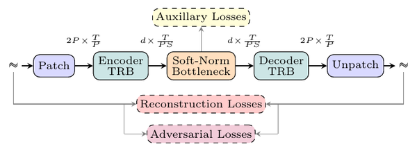
| ~1.4B flow-matching DiT, fixed 50k-step budget | VAE vs soft-normalization bottleneck (fixed normalization statistics in place of a sampled posterior), both at 4096x temporal downsampling, 256-dim | identical (MELlog1p 0.108 for both) | FAD-CLAP 0.651 vs 1.061 | SAME, Table 2, p. 8 |
| same | conventional 1024x/64-dim VAE vs auxiliary-loss-shaped 4096x/256-dim | best in the table (0.098) vs 0.109 | 0.724 vs 0.576 | SAME, Table 2, p. 8 |
| 1B TTS DiT retrained per VAE | latent dimension 64 to 256 at fixed 20 Hz | STOI, speaker similarity, and PESQ improve; UTMOS dips | TTS WER, UTMOS, DNSMOS all degrade | LongCat-AudioDiT, Sec. 5.3.2, Fig. 3 |
| one text-to-sound diffusion model | KL target swept across a 7.65–74.10 kbps family | rises with bitrate along the rate-distortion curve (Fig. 1) | peaks at 11.56 kbps (text-audio similarity 70.67, KAD 1.70), degraded at 74.10 kbps (66.84, 2.16) | Target-KL, Table 2 |
| F5-TTS Small | vanilla VAE vs the same VAE aligned to WavLM, a self-supervised speech representation model; both 40 Hz/64-dim | equivalent (PESQ 3.75 vs 3.74) | WER 2.65 vs 1.95, SIM 0.60 vs 0.64 | Semantic-VAE, Tables 1-2 |
The first two rows come from one SAME ablation. Metrics: MELlog1p is a multi-resolution log-mel reconstruction distance (lower is better); FAD-CLAP is Fréchet audio distance in the embedding space of CLAP, a contrastive audio-text model (lower is better); STOI is a 0–1 intelligibility measure and PESQ a reference-based speech quality score, both computed against the original audio; WER is word error rate of an ASR model run on the synthesized speech; UTMOS and DNSMOS are model-predicted mean-opinion quality scores; text-audio similarity is a CLAP-embedding match score and KAD a kernel-based distribution distance between real and generated audio embeddings; SIM is speaker similarity, the cosine between speaker-embedding vectors.
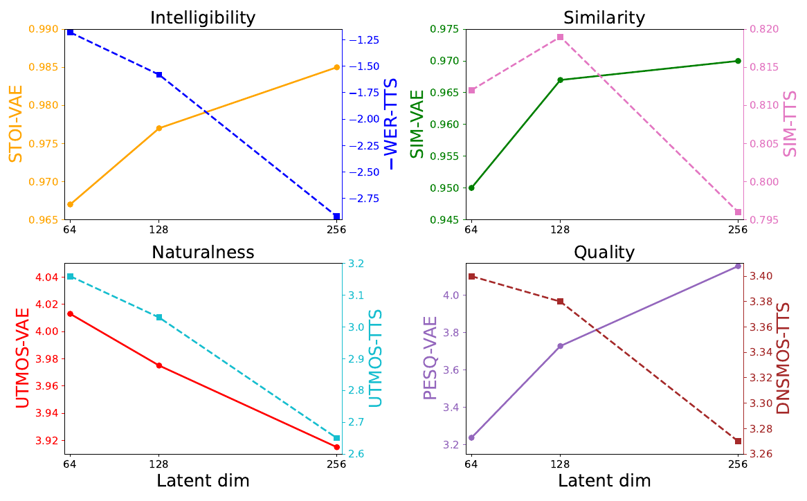
LongCat-AudioDiT, Figure 3, p. 11. Solid lines are the Wav-VAE's reconstruction metrics, dashed lines the paired TTS model's, against latent dimension; the intelligibility panel plots negated WER, so falling means worse. The decoupling is sharpest in the intelligibility and quality panels; TTS speaker similarity peaks at 128 before dropping at 256, and the naturalness metrics decline on both sides.
The rows differ in what they isolate. The SAME pair puts the disagreement in distributional structure that the bottleneck's fixed statistics do not capture; the SAME post traces which auxiliary losses put that structure in. LongCat shows the failure is not a generator-capacity problem: aside from a marginal speaker-similarity gain, scaling the TTS backbone to 3.5B on the 128-dim VAE still loses to 3.5B on the 64-dim VAE, so under a fixed training recipe the extra width is a modeling burden that added parameters do not offset. Target-KL shows the disagreement inside a single architecture family swept along one axis, which rules out confounds between recipes. And Semantic-VAE shows the converse: a latent change that improves generation substantially while reconstruction does not move at all.
The direction of the trade is not universal: AudioLDM's mel-spectrogram VAE reconstructs comparably across its compression sweep while generation quality falls as compression rises, the opposite of LongCat's frame-rate result below, so the optimum is task- and architecture-dependent. The durable conclusion is the selection rule: only a paired downstream model ranks latents as generation targets. Every sweep above paid for a full generator per candidate; whether a small jointly trained probe would produce the same ranking at a fraction of the cost is untested.
Frame rate and width set the prediction problem
Frame rate and channel width are fixed before any training loss applies, and they define the object the generator must predict: rate sets the sequence length and how much information each step carries, width sets the dimensionality of the continuous vector the diffusion head or distribution predictor must model per step. Sequence length is what an autoregressive generator pays for in context and compute, which is why long-form TTS systems push rates down to 7.5–15 Hz; the VibeVoice post works out that budget arithmetic. The two axes convert: in LatentLM's compression ablation, dropping the frame rate from 37.5 to 15 Hz at fixed width costs reconstruction similarity (0.866 to 0.700), and doubling the width restores it (0.870), with downstream TTS similarity following the same pattern. Information removed from the time axis must be carried by added latent dimensions.
Two sweeps locate the best shape for autoregressive speech at the same information rate, 480 floats per second:
| Sweep (both at 480 floats/s) | 3.75 Hz | 7.5 Hz | 15 Hz | 30 Hz | 60 Hz |
|---|---|---|---|---|---|
| LatentLM: TTS speaker similarity (dims 128/64/32) | 0.598 | 0.656 | 0.697 | ||
| SemaVoice: TTS word error rate % (dims 32/16/8) | 2.97 | 3.24 | 14.71 |
LatentLM, Tables 4-5; SemaVoice, Table 4. LatentLM sweeps downward from 15 Hz and loses speaker similarity as the rate falls; SemaVoice sweeps upward and loses intelligibility as the rate rises, while its reconstruction stays roughly stable. Jointly the two bracket 15 Hz as the optimum at this budget, approached from opposite directions; the sweeps differ in data, benchmark, backbone, and head, so they do not trace a controlled curve. And because the budget is fixed, rate and width move together: the 60 Hz failure happens in 8-dim frames, so the high end cannot separate a rate ceiling from a width floor. LongCat's rate sweep points the same way from the non-autoregressive side: lowering the frame rate at fixed dimension 64 costs VAE reconstruction similarity and PESQ while improving the paired TTS model, except for TTS speaker similarity, which peaks at 11.72 Hz, the rate LongCat ships.
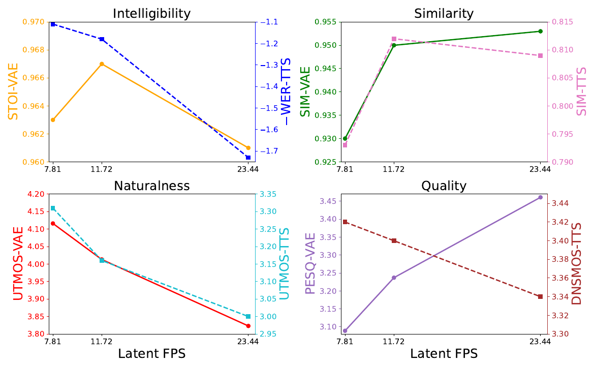
LongCat-AudioDiT, Figure 4, p. 12. Solid lines are the Wav-VAE's reconstruction metrics, dashed lines the paired TTS model's, against latent frame rate; the quality panel shows the two moving in opposite directions, and the similarity panel the TTS peak at the middle rate.
Width gets two defensible answers. LongCat's response to its dimension sweep is to keep the latent narrow, 64-dim at 11.72 Hz. SAME keeps a wide 256-dim latent at a frame rate close to LongCat's and restores predictability with auxiliary semantic and generation losses. LongCat's sweep varies width alone and measures the cost of raw width; SAME demonstrates that shaped width is usable, though its own table complicates a pure width story: the unshaped wide VAE already beats the narrow configuration on generation, a comparison that confounds width with frame rate. No source varies width and shaping independently. Geometry beyond the uniform time grid is also in play: Music2Latent2 packs each audio chunk into a set of unordered summary embeddings so global features are not re-encoded at every frame, and TADA collapses 50 Hz frames into one vector per text token, trading the time grid for text alignment.
Regularization decides which component absorbs prediction error
A predicted latent is always slightly off the encoder's output manifold. Regularization choices decide which component absorbs that error, and the systems here give four answers that shipping recipes combine.
The latent distribution absorbs it. A vanilla VAE lets per-channel posterior variances collapse toward zero, leaving sampled latents brittle as autoregressive context. A sigma-VAE takes the variance out of the encoder's hands, training the decoder and the generator under latent noise of a designed scale so that prediction errors smaller than that scale stay in-distribution; the exposure bias post develops the mechanism and its evidence. LatentLM, VibeVoice, and SemaVoice all build their speech tokenizers on the recipe.
The decoder absorbs it. Injecting Gaussian noise into latents during autoencoder training builds the same robustness into a different component, and it is nearly free. LatentFlowSR's ablation isolates the effect: under inference-time latent noise its plain autoencoder collapses (LSD 3.42, ViSQOL 2.36, where LSD is log-spectral distance, lower better, and ViSQOL a 1–5 perceptual quality estimate) while the noise-trained version barely moves (0.92, 4.22), and on clean audio the noise-trained autoencoder reconstructs slightly better, not worse. SAME trains with latent noise at 5e-2 and keeps a smaller 1e-3 noise on the latent at inference.
The generator absorbs it. An under-regularized latent reconstructs well but is sharp and perturbation-sensitive, so the full difficulty lands on the predictor; an over-regularized latent is smooth but caps fidelity. Most recipes pick a point on that trade implicitly through an ad hoc KL weight (Stable Audio Open down-weights KL by 1e-4 and accepts whatever rate emerges); Target-KL replaces the weight with a specified information rate, a squared penalty pulling measured KL toward a chosen value, which is what made the sweep in the table above possible. Its TTS results carry one caveat: some high-bitrate VAEs scored deceptively low WER because the diffusion model copied information from unregularized prompt latents, with monotonous-sounding output. KALL-E occupies the deliberately smooth end, keeping a high KL weight (32) and accepting worse reconstruction for a latent its autoregressive distribution predictor can fit.
A separate pathway absorbs it. VibeVoice routes semantics around the generated latent entirely: its acoustic tokenizer stays purely reconstructive, and at each step a frozen ASR-trained encoder re-encodes the audio just generated and adds the result to the autoregressive history.
SAME goes one step further: rather than only making errors survivable, it trains a small flow-matching model jointly with the encoder and backpropagates that model's loss, so the latent space itself is optimized to be easy for a generator to model. The SAME post covers the mechanism; flow matching is the objective both that probe and most of the downstream generators here train with.
Semantic alignment strength must match latent capacity
Semantic objectives change what the latent encodes rather than how much, and whether they conflict with acoustic fidelity depends on the alignment's strength and the latent's capacity, not on semantic alignment per se.
A hard semantic objective on a small bottleneck degrades both sides. VibeVoice pushed a full transcript-decoding ASR objective through a 7.5 Hz, 64-dim latent and collapsed reconstruction and speaker similarity together (PESQ 1.92 against 2.98 for its reconstruction-only tokenizer); the mechanism, two objectives competing for fixed capacity, is analyzed in the VibeVoice post. The WER Trap measures the same competition from the semantic side with a discrete 5 Hz ASR-supervised token: adding a reconstruction loss costs character error rate (11.98 to 14.32) and audio-QA accuracy. Both land on decoupling the objectives.
A gradient-bounded alignment loss improves both sides. SemaVoice aligns its 15 Hz latent to frozen WavLM features with a frame-wise cosine loss plus a pairwise self-similarity loss, and sets the alignment weight each step so its gradient norm is half the reconstruction loss's, so the alignment can never dominate. It improves WER and speaker similarity together, costs almost nothing on reconstruction, and its value grows with frame rate: at 60 Hz, where the aligned sweep has already degraded to WER 14.71, removing the alignment doubles the damage to 28.06. Loss form matters as much as weight: in Semantic-VAE, cosine alignment to a late WavLM layer improves TTS, while L1 and MSE alignment to the same teacher are worse than no alignment at all (WER 3.12 and 4.37 against the 2.65 baseline); magnitude-constraining losses over-restrict the latent where directional alignment only orients it. CALM extends to its full continuous latent the WavLM cosine distillation that Mimi, the discrete tokenizer it derives from, applies only to its first codebook.
A weak objective on a wide latent is nearly free. SAME applies linear probes regressing DSP features plus a contrastive text critic to its 256-dim latent and takes the best generation scores in its ablation at a small reconstruction cost. The availability of a teacher explains why the recipes differ across domains: speech has WavLM-class self-supervised content teachers, so SemaVoice, Semantic-VAE, and CALM align to them; music has no equivalent, so SAME builds its semantic targets from the signal (chromagrams, interaural level difference) and from paired text. No single source varies alignment strength at fixed rate and width, so where soft becomes hard, and how width moves that threshold, remains unmeasured.
Staged training routes adversarial gradients away from the encoder
The sources here disagree about freezing schedules but agree about routing: losses that shape the latent for generation (semantic alignment, SAME's diffusion probe) are deliberately sent into the encoder, while adversarial and feature-matching gradients that fit fine-grained waveform detail are kept off it during late fine-tuning. RAVE shows why: it trains its VAE for representation first, then freezes the encoder and fine-tunes only the decoder adversarially, and its appendix shows that letting the stage-two feature-matching loss reach the encoder dramatically inflates the latent space's estimated dimensionality (by SVD, its 128 nominal dimensions hold about 16–24 informative ones when the encoder is protected). RAVE measures the harm as lost compactness, not generation quality, but spreading information across more dimensions is exactly the raw width whose cost the LongCat sweep measured. The pattern at scale: Stable Audio Open trains end to end with adversarial losses for 183 hours, then spends 273 hours training the decoder alone against a frozen encoder, and SAME freezes its encoder for two decoder-only stages.
Sources
- SAME: A Semantically-Aligned Music Autoencoder: the fixed-budget bottleneck ablation rows in the decoupling table (Table 2, Sec. 5.1); noise injection scales (Sec. 2.3); the linear-probe and contrastive losses and the joint diffusion probe (Sec. 3.3); frozen-encoder decoder stages (Sec. 4.2).
- LongCat-AudioDiT: High-Fidelity Diffusion Text-to-Speech in the Waveform Latent Space: the dimension and frame-rate sweeps with paired TTS models, the 3.5B scaling check, and Figures 3 and 4 (Sec. 5.3.2, pp. 11-12).
- Taming Audio VAEs via Target-KL Regularization: target-KL as a specified information rate (Secs. 1-2), the rate-distortion curve (Fig. 1), the text-to-sound generation peak and the TTS prompt-copying caveat (Tables 2-3, Sec. 4).
- Semantic-VAE: Semantic-Alignment Latent Representation for Better Speech Synthesis: reconstruction-equivalent VAEs with diverging F5-TTS results (Tables 1-2) and the cosine/L1/MSE loss-form ablation (Table 3).
- Multimodal Latent Language Modeling with Next-Token Diffusion (LatentLM): the sigma-VAE recipe (Sec. 2.3), the frame-rate sweep (Tables 4-5), and the compression/width conversion ablation (Table 6).
- SemaVoice: Semantic-Aware Continuous Autoregressive Speech Synthesis: the gradient-ratio-capped WavLM alignment (Eqs. 3-7) and the granularity sweep with and without alignment (Table 4).
- VibeVoice Technical Report: the coupled-tokenizer collapse, the hybrid acoustic/semantic routing, and the semantic feedback path (Tables 5 and 7, Appendices B and D).
- The WER Trap: the reconstruction/semantics competition measured from the discrete-token side (Tables 1-2).
- LatentFlowSR: High-Fidelity Audio Super-Resolution via Noise-Robust Latent Flow Matching: the latent-noise-injection robustness ablation (Tables 4-5).
- RAVE: A Variational Autoencoder for Fast and High-Quality Neural Audio Synthesis: two-stage training with the frozen encoder (Sec. 3.1.2), the SVD dimensionality estimate (Sec. 5.3, Fig. 2), and the unfrozen-encoder dimensionality inflation (Annex E, Fig. 8).
- Stable Audio Open: the standard loss substrate, the 1e-4 KL weight, and the joint/frozen-phase compute split (Sec. 2).
- AudioLDM: Text-to-Audio Generation with Latent Diffusion Models: the compression-level sweep where reconstruction holds and generation degrades (Tables 4 and 8).
- KALL-E: Autoregressive Speech Synthesis with Next-Distribution Prediction: the deliberately high KL weight and its stated rationale (experimental setup and Table 1 discussion).
- Music2Latent2: Audio Compression with Summary Embeddings and Autoregressive Decoding: unordered summary embeddings (Secs. 1-3).
- TADA: A Generative Framework for Speech Modeling via Text-Acoustic Dual Alignment: text-token-aligned acoustic vectors (Sec. 3).
- Continuous Audio Language Models (CALM): WavLM distillation over the full continuous speech latent, contrasted with Mimi's first-codebook distillation (Sec. 4.1).
Related Diffio posts
- SAME Makes Generation Difficulty an Autoencoder Training Loss: the single-system deep dive on shaping a latent with a jointly trained generation probe.
- VibeVoice: Frame Rate Is the Context Budget for Long-Form TTS: the frame-rate budget arithmetic and the coupled-tokenizer capacity analysis.
- Exposure Bias: Corrupt the Context, Keep the Target Correct: why autoregressive consumption makes latent variance an error-tolerance radius.
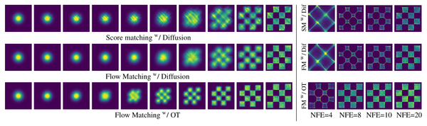
- Flow Matching: Regress the Field the Sampler Integrates: the training objective of most generators these latents are built for.
- TTS Models: A Map Of The Modern Speech Stack: where continuous-latent systems sit among the TTS architecture families.