SAME Makes Generation Difficulty an Autoencoder Training Loss
SAME (Semantically-Aligned Music autoEncoder) is Stability AI's autoencoder for 44.1 kHz stereo music and general audio, and the frozen latent space that Stable Audio 3, the company's text-to-audio generator family, generates in. It compresses the waveform 4096x along the time axis into 256-dimensional latent frames at roughly 10.8 Hz, about twice the temporal compression of recent audio VAEs at four times their usual 64 channels. Two variants are released as open weights, SAME-L and the CPU-targeted SAME-S. The design problem at this operating point is producing a latent distribution that a flow-matching generator can learn, not reconstruction, and SAME attacks it directly: a small diffusion transformer trains jointly with the autoencoder on its latents, and its loss backpropagates into the encoder. In the paper's controlled ablation the auxiliary losses are load-bearing: the deterministic bottleneck they accompany is, alone, worse than the VAE it replaces, and with them it is better.
A 4x shorter, 4x wider latent at the same scalar rate
Raising temporal downsampling shortens the sequence a downstream generator must model; at fixed latent dimension it also raises compression difficulty, so SAME widens the latent to compensate. At 10.8 Hz and 256 channels the latent carries about 2,760 floats per second, exactly the scalar rate of a conventional 1024x, 64-channel audio VAE: the budget is unchanged, reshaped into a 4x shorter, 4x wider sequence, because sequence length is what a generator pays for in compute and context. A 6-minute track is about 3,900 latent frames. Early latent-diffusion practice kept latent dimension small on the belief that wide latents are hard to generate in; SAME instead cites the representation-autoencoder (RAE) results from images, where large dimensions are tractable when the latent is semantically structured.
Patching and transformer resampling replace strided convolution

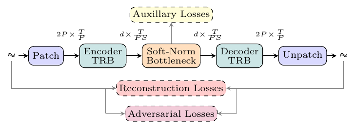
SAME paper, Figure 1, p. 2. The auxiliary losses attach at the bottleneck, on the latent itself; the reconstruction and adversarial losses act on the decoded waveform.
There are no learned convolutions on the signal path. A parameter-free patching pretransform reshapes stereo waveform (B, 2, T) into (B, 2P, T/P) with P=256, so each embedding concatenates 256 left-channel and 256 right-channel samples: 256x downsampling as a pure reshape. The remaining 16x comes from a Transformer Resampling Block (TRB): the patch sequence is partitioned into non-overlapping 16-embedding segments, one learnable output embedding is appended to each, a transformer stack processes the interleaved sequence, and only the output embeddings are kept. The decoder TRB reverses the roles, pairing each latent with 16 learnable outputs.

SAME paper, Figure 2, p. 3, shown with stride 2 for clarity; the released models use stride 16. Downsampling happens through attention into one learned token per segment, not through pooling or strided convolution.
In SAME-L the transformer layers use differential attention with RoPE and per-head QK-normalization, and the last 8 decoder layers swap their feed-forward activations for sin(pi x), a periodic basis for waveform detail; SAME-S drops both for CPU throughput. Both variants replace LayerNorm with Dynamic Tanh, a learnable tanh activation, avoiding normalization statistics that near-silent audio segments corrupt. Because training segments are a few seconds but inference must handle arbitrary lengths, full attention is unsuitable: SAME-L uses sliding-window attention, and SAME-S uses chunked attention whose chunk grid shifts by half a chunk midway through the stack, so first-half chunk boundaries fall in second-half chunk interiors and stop producing audible boundary artifacts; CPU inference libraries such as LiteRT do not support sliding windows. The all-transformer design buys speed: SAME-L runs at about twice the real-time factor (audio duration over encode-plus-decode wall clock) of smaller convolutional VAE baselines despite its 852M parameters, which the paper attributes to well-optimized transformer primitives plus the high compression ratio.
Soft-normalization: a deterministic bottleneck that pins statistics
Where most continuous audio codecs put a VAE, SAME puts a deterministic normalization with no sampled posterior. The encoder output passes through a learnable per-channel affine transform, then is divided by a running standard deviation tracked by exponential moving average. A penalty of Gaussian KL form pushes means and variances toward zero and one along two axes independently, per channel over time and per timestep across channels, so neither individual channels nor individual frames drift to extreme statistics. Gaussian noise scaled by the running standard deviation is added to the latent (5e-2 during training, 1e-3 at inference), smoothing the latent manifold so the decoder tolerates the imperfect latents a downstream generator will hand it.
L_diff: an auxiliary diffusion model trains jointly and backpropagates into the encoder
When building discrete tokenizers it is common to jointly train a small autoregressive prior whose loss backpropagates into the encoder, keeping the token distribution easy for that prior to model; for continuous latents under diffusion the paper calls the equivalent move rarer, citing a single recent precedent. SAME's version is the loss it calls L_diff: a 4-layer, 768-dimensional diffusion transformer trains on the latents with the standard straight-path flow-matching objective, noising z_t = (1-t)z + t*eps and regressing the velocity eps - z, with timesteps drawn from a truncated logistic-normal distribution. The auxiliary model warms up on detached latents; after warmup, its gradients flow into the encoder.
The auxiliary model is unconditional and exists only as a training signal. L_diff rises when the current latent distribution is hard for a flow-matching model to fit, so minimizing it with respect to the encoder pushes the latent toward geometries that are easier to generate in. An unconditional model this small is a coarse proxy for the text-conditioned generator that will actually use the latent; Stable Audio 3 pre-trains on the same frozen latents with the same straight-path velocity parameterization (its full objective adds minibatch optimal-transport coupling and an inpainting mask), so the encoder is shaped during its own training by a scaled-down version of the downstream generator.
L_sem and L_con: linear chroma and stereo regressors, plus a contrastive text critic
Speech tokenizers usually buy semantic structure by aligning the latent to a self-supervised teacher such as WavLM. SAME aligns to no pretrained teacher; its semantic regression loss, L_sem, supervises with quantities computed from the signal itself. Single 1x1-convolution regressors predict three octave-banded chromagrams (per-frame energy by pitch class) and an interaural level difference (the per-band left/right log-magnitude gap that encodes the stereo image) directly from the latent; because the regressors are linear, pitch-class and spatial structure are pressured to stay linearly decodable rather than nonlinearly entangled. A separate contrastive loss, L_con, trains a critic to score whether a latent sequence, a wavelet decomposition of the audio, and a T5Gemma embedding of the paired text description come from the same input, with negatives formed by re-pairing audio and text within the batch and heavy masking of latent and feature positions to block shortcut cues. Like the auxiliary diffusion model, the critic warms up on detached latents before its gradients reach the encoder.
The pressure is mild: linear regressors and a warmed-up critic on a 256-dimensional latent. VibeVoice found that the opposite setting, a hard transcript-decoding objective pushed through a 7.5 Hz, 64-dimensional speech latent, degraded reconstruction and collapsed speaker similarity.
The bottleneck ablation: reconstruction pinned, generation decoupled
The ablation holds everything fixed except the latent space: 50k autoencoder steps with the SAME-L backbone and no adversarial losses (removing GAN dynamics as a confounder), then a roughly 1.4B-parameter diffusion transformer (DiT) trained with flow matching on each latent space for 50k steps. VAE variants use a single, unswept KL weight (1e-4). Both budgets are short, so the comparison measures how readily a DiT fits each latent space at fixed compute, not converged quality.
| Config | Compression / width | Bottleneck | MELlog1p (recon) | FAD-CLAP (gen) | MuQEval (gen) |
|---|---|---|---|---|---|
| A | 4096x / 256 | VAE | 0.108 | 0.651 | 3.252 |
| B | 4096x / 256 | soft-norm | 0.108 | 1.061 | 2.783 |
| C | 4096x / 256 | soft-norm + L_diff | 0.103 | 0.593 | 3.340 |
| D | 4096x / 256 | soft-norm + L_diff + L_sem/L_con | 0.109 | 0.576 | 3.870 |
| E | 1024x / 64 | VAE | 0.098 | 0.724 | 3.194 |
SAME paper, Table 2, p. 8. MELlog1p is a multi-resolution log-mel reconstruction error (lower is better); FAD-CLAP is Fréchet audio distance in the embedding space of CLAP, a contrastive audio-text model, computed on the DiT's caption-conditioned outputs (lower is better); MuQEval is a model-based, reference-less musical quality score (higher is better).
Configs A and B reconstruct identically on the table's metric and generate very differently: FAD-CLAP 0.651 against 1.061. The statistics soft-normalization pins (means, variances, magnitudes) survived the swap, so whatever the DiT needed lives in distributional structure beyond those statistics, which a reconstruction metric cannot see. Adding the auxiliary diffusion model (config C) more than repays the simplification, beating the VAE baseline on all three metrics at no reconstruction cost; the table cannot say whether the gain is diffusion-specific shaping or a more generic smoothing pressure, and the untested VAE-plus-L_diff cell is what would separate the bottleneck's contribution from the auxiliary model's. Adding the semantic losses (config D) trades a little reconstruction for the best generation scores, with a MuQEval jump the paper reads as musical structure becoming easier to model; L_sem and L_con are added together, so their individual contributions are unknown.
Config E is the conventional 1024x/64 shape: the table's best reconstruction, and worse generation than A, C, and D. All generation evidence in the paper is this internal ablation; no generator is trained on a competitor's latent space. The same reconstruction/generation decoupling has been measured independently across speech and audio systems.
Full-scale reconstruction: best mel error and listening score from a 4x shorter sequence
The released models train in three stages on about 19,500 hours of licensed production audio (a 66/25/9 percent music, sound-effects, instrument-stems mix): an end-to-end stage with all losses, then two decoder-only stages with the encoder frozen, the second swapping in a transformer-based discriminator ensemble and synthetic linear frequency sweeps against aliasing.
| Metric | eps-ar-VAE | ACE-Step 1.5 | SAO VAE | CoDiCodec | SAME-S | SAME-L |
|---|---|---|---|---|---|---|
| Compression | 1024x | 1920x | 2048x | 4096x | 4096x | 4096x |
| Latent dim | 64 | 64 | 64 | 64 | 256 | 256 |
| RTF | 325 | 284 | 300 | 47 | 2069 | 561 |
| SI-SDR | 12.0 | 7.0 | 6.2 | -0.3 | 9.6 | 11.9 |
| STFTlog1p | 0.080 | 0.084 | 0.092 | 0.096 | 0.088 | 0.081 |
| MELlog1p | 0.070 | 0.069 | 0.079 | 0.096 | 0.071 | 0.057 |
| CCPC | 97.2 | 93.2 | 92.2 | 81.7 | 95.5 | 96.6 |
| MUSHRA | 77.6 | 76.5 | 73.3 | n/a | 66.1 | 82.2 |
SAME paper, Table 1, p. 8; baselines are recent open-weights continuous audio autoencoders. Objective metrics use 446 captioned music tracks from the Song Describer Dataset: SI-SDR is scale-invariant signal-to-distortion ratio in dB (higher is better), STFTlog1p a log-magnitude STFT distance (lower is better), CCPC cross-channel phase coherence for stereo-image fidelity (higher is better). RTF is averaged over 50 two-minute tracks, FP16 on one H100. MUSHRA is a 0-100 listening test on excerpts, here 36 valid trials from 12 participants after filtering, with the hidden reference (the clean original, rated blind) at 97.6; CoDiCodec was excluded from it.
SAME-L takes the best mel error and the best mean listening score (82.2 against 77.6 for the strongest baseline, with overlapping confidence intervals), while eps-ar-VAE, the conventional 1024x/64 shape, stays marginally ahead on SI-SDR, the magnitude-STFT distance, and stereo phase coherence. Every number here is music reconstruction; despite the sound-effects share in training, non-music quality is never evaluated in the paper.
SAME-S, the 108M CPU variant, matches the Stable Audio Open VAE on objective reconstruction at 6-7x the speed; its listening score is lower (66.1 to SAO's 73.3). Its distillation aligns student latents to the frozen SAME-L teacher's with an L1 loss and applies reconstruction and adversarial losses to cross-decoded outputs, student decoder on teacher latents and the reverse, so the two models share one latent space with interchangeable latents. That is what lets Stable Audio 3 train its small model on SAME-S and its larger models on SAME-L.
Sources
- SAME: A Semantically-Aligned Music Autoencoder: all architecture and training details (Secs. 2-4), the bottleneck ablation (Table 2, Sec. 5.1), reconstruction and MUSHRA results (Table 1, Secs. 5.3-5.4), Figures 1 and 2.
- Stable Audio 3: the generator trained on SAME latents; model tiers on SAME-S/SAME-L and the flow-matching pre-training objective (Secs. 2.1, 3.2).
- Diffusion Transformers with Representation Autoencoders: the image-domain wide-latent argument SAME cites for choosing d=256.
- SAME open weights and audio examples