TTS Models: Sampled Acoustic Representations Set the Generator Constraints
A map of modern text-to-speech systems by the representation their generators sample: codec tokens, mel frames, semantic-acoustic cascades, continuous latents, and hybrid frames.
Modern text-to-speech systems are easiest to place by naming the representation the primary acoustic generator samples before waveform rendering. A paper may call the model a codec language model, a diffusion TTS model, a speech LLM, or a flow-matching system, but the more durable question is what representation the system is trying to sample and on what schedule.
The prediction target is the first generator constraint. It strongly shapes the loss family, the sampler, the latency path, the representation boundary, and the kinds of errors that can compound at inference time. A generator that emits token IDs learns a categorical distribution. A generator that samples mel frames works over a continuous acoustic field, even if the network head predicts velocity or noise rather than the frame itself. A generator that emits semantic tokens still needs another model to render timbre, timing, prosody, and residual acoustic detail. A generator that emits continuous latents needs a sampler and a latent space that remain stable under prediction.
Backbone choice matters, but many recent TTS systems share familiar Transformer, DiT, Llama, Qwen, Ministral, or flow-matching machinery. The clearer first map is by sampled representation, with generation schedule tracked beside it.
The sampled representation constrains the generator
For multi-stage systems, track both the long-range sampled representation and the local acoustic-rendering representation. The sampled representation is neither the final waveform nor every internal tensor predicted by a neural network head. It is the representation that carries the acoustic modeling burden before a vocoder or codec decoder turns it into waveform.
Generation schedule is the second classification axis. Autoregressive, masked, non-autoregressive, delay-pattern, within-frame residual-depth, and ODE samplers create different critical paths over the same representation. Frame rate is not the same thing as total work or total bitrate.
| Sampled representation before waveform rendering | Generator constraint | Typical systems | Primary design constraint |
|---|---|---|---|
| Discrete codec token IDs | Sample codebook indices with a softmax, often across residual vector quantization depth | VALL-E, SoundStorm-style acoustic token stages, MOSS-TTS | Token rate, codebook depth, codec quality, generation schedule, and exposure to token errors |
| Continuous acoustic frames | Sample mel-spectrogram frames, often by predicting a vector field over those frames | Voicebox, Matcha-TTS, F5-TTS | Duration, alignment, ODE or diffusion step count, and vocoder quality |
| Semantic tokens followed by acoustic rendering | First sample content-biased units, then synthesize acoustic detail from them | CosyVoice, MaskGCT | Whether semantic tokens preserve enough lexical content, speech timing, prosody, and speaker information |
| Continuous latent vectors | Sample vectors from a learned low-rate audio latent space | LatentLM, VibeVoice, SemaVoice | Latent geometry, frame rate, vector width, variance modeling, and sampler robustness |
| Mixed per-frame bundles | Sample a low-rate semantic stream plus local acoustic variables inside each frame | Voxtral TTS, recent codec-LLM hybrids | How much global structure stays autoregressive and how much acoustic detail is delegated to a local generator |
The table separates sampled representations and sampler choices rather than ranking systems. A "language model" over audio can mean token IDs, continuous vectors, semantic codes, or a mixed frame. A "diffusion" or "flow" model can be the main generator, the acoustic renderer, or a local head attached to a token model. Semantic tokens are content-biased but can retain speaker and prosodic information.
Discrete codec tokens make TTS a categorical sequence-modeling problem
Discrete codec TTS makes speech look like language modeling. A neural codec converts waveform into a grid of codebook IDs. The generator predicts those IDs, and the decoder converts a legal code stack back into audio.
VALL-E is the canonical version of this setup. It uses an EnCodec representation with 75 frames per second and eight residual vector quantization codebooks. VALL-E predicts the first codebook autoregressively and fills the remaining codebooks with non-autoregressive models.
Discrete codec tokens let the generator use cross-entropy, prompting, and sampling temperature, but quality and controllability remain bounded by codec rate, residual depth, and decoder behavior. A correct-looking token sequence can still sound wrong if the codec does not preserve the cue the task needs.
MOSS-TTS is the low-frame-rate, high-RVQ-depth case. It lowers the sequential frame rate to 12.5 frames per second while increasing residual quantization depth to 32 layers. That does not make acoustic modeling cost disappear. It changes the critical path from many temporal decisions to fewer temporal decisions with deeper within-frame reconstruction.
The codec-token design choice is how to allocate modeling capacity across temporal steps, residual codebooks, and within-frame decoding. Once the time axis is compressed, autoregressive temporal prediction is only one part of the problem. The model must also predict the residual-depth position within each frame.
Mel-frame systems generate continuous acoustic features
Mel-frame systems leave discrete neural codec tokens out of the acoustic generator's sampled representation. The target is a dense time-frequency representation, usually an 80- or 100-bin log-mel frame sequence, and a separate vocoder turns that representation into waveform. The vocoder is not neutral: mel targets discard phase and rely on the vocoder prior for final waveform detail.
Voicebox, Matcha-TTS, and F5-TTS generate log-mel frames with non-autoregressive flow-matching models before a vocoder. Voicebox uses 80-dimensional log-mel frames at 100 Hz, and F5-TTS uses 100-channel log-mel frames before Vocos. Their inference cost is controlled by the number of function evaluations, or NFEs, rather than by autoregressive token count.
The model samples continuous acoustic features before vocoding. This avoids dependence on a codec codebook layout, but duration, alignment, conditioning, vector-field sampling, and vocoder behavior remain part of the design.
For TTS, flow matching shifts the design problem from vocabulary construction to vector-field modeling.
Semantic-token cascades separate content modeling from acoustic rendering
Semantic-token systems factor speech generation into semantic-token prediction and acoustic rendering. First, sample a content-biased representation. Then, render acoustics from that representation plus speaker, prompt, style, or text conditioning. "Semantic" can mean ASR-supervised units, self-supervised clusters, phoneme-like codes, or a semantic branch inside a codec.
CosyVoice is a representative supervised version. It extracts semantic tokens from an ASR-oriented model, uses a language model to generate those tokens from text, then uses a flow-matching acoustic model and HiFi-GAN vocoder to synthesize speech. MaskGCT is a masked-generation version: it uses a semantic tokenizer for content and an acoustic codec for waveform detail, then generates both stages with iterative masked prediction rather than a single left-to-right token pass.
The appeal is modularity. Text correctness and acoustic rendering are no longer forced into one token stream. Semantic tokens reduce the sequence length between text conditioning and acoustic rendering by replacing waveform-length acoustic detail with lower-rate content-biased units. The acoustic model can then focus on speaker identity, pitch, rhythm, and fine acoustic detail.
WER can overstate a semantic tokenizer's suitability for generative TTS. Word error rate, or WER, measures lexical recoverability but not whether the tokens preserve timing and acoustic correlations needed by a generator. The WER Trap paper shows speech tokens can score well on ASR-like tests while still failing to preserve the acoustic variation a generator needs. It proposes flow-probe diagnostics that ask whether a flow model can reconstruct acoustic trajectories from the tokens, not just whether an external recognizer can read them.
The generator constraint for a semantic cascade is two-sided. The first stage must preserve enough content to guide the utterance, and the second stage must be able to recover the missing acoustics without inventing the wrong speaker, rhythm, or affect.
Continuous latents replace codebook indices with vector prediction targets
Continuous-latent TTS removes the categorical codebook interface. Instead of sampling token IDs, the generator samples vectors from a learned audio latent space. These are not just mel frames with a different name: mel bins are hand-designed acoustic features, while continuous latents are learned compressed vectors intended to be reconstructable and predictable. That makes the sampled representation a regression, diffusion, or flow problem rather than a softmax problem.
LatentLM is the cleanest general statement of this idea. It replaces next-token classification with next-token diffusion over continuous latents. For speech synthesis, it evaluates low-rate speech latents down to 3.75 Hz, making the context length look more like text while keeping the prediction target continuous.
VibeVoice is the long-form TTS example: a 7.5 Hz continuous acoustic latent plus a next-token diffusion head shifts the budget from sequence length to latent geometry. Its coupled shared-latent tokenizer ablation reduces perceptual speech quality (PESQ) and objective speaker similarity (SIM-O), which is why the related VibeVoice and latent-encoder posts treat rate, width, variance, and semantic alignment as generator constraints.
SemaVoice makes the same point from another direction. It uses continuous speech tokens at 15 Hz, and its frame-rate study shows that simply increasing temporal resolution is not automatically better. The denser 60 Hz setup degrades sharply in that study, especially without alignment. Without the right alignment and capacity, a denser latent stream can make prediction harder rather than easier.
A representation is both a compression format and the target distribution the generator must learn.
Hybrid frames combine autoregressive semantic tokens with local acoustic generation
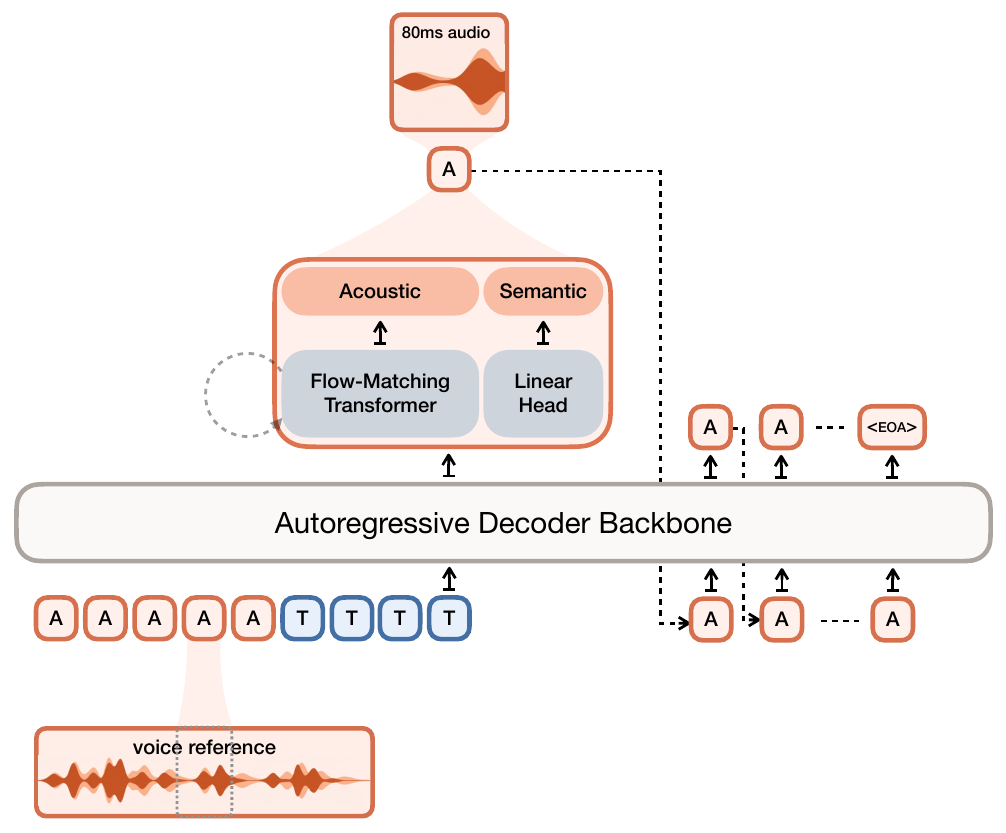
Recent systems increasingly combine the earlier choices rather than choosing only one. Voxtral TTS is a useful marker. Its codec runs at 12.5 Hz and represents each frame with one 8192-entry semantic VQ token plus 36 finite-scalar-quantized acoustic coordinates. The decoder backbone generates the semantic stream autoregressively. A flow-matching acoustic head models those 36 acoustic coordinates in continuous space, runs eight NFEs by default, then discretizes the result back to the 21-level FSQ interface.

Voxtral combines a codec representation with a flow-matching acoustic head. The semantic stream keeps a language-model-style global ordering. The acoustic head avoids making all fine acoustic detail a long sequence of categorical decisions. Streaming then becomes a coordination problem between the autoregressive semantic loop, the local acoustic generator, and the audio decoder.
MOSS and Voxtral address the same residual acoustic modeling problem with different allocations: MOSS models RVQ depth within each frame, while Voxtral models local acoustic coordinates with a per-frame flow model. VibeVoice offers another answer by keeping the low-rate acoustic representation continuous.
Reducing sequential frame rate relocates acoustic detail into residual depth, a semantic-acoustic cascade, a local flow head, a mel-frame sampler, or a continuous latent space.
Five fields locate a TTS system
A new TTS system can be classified by five fields.
- Which representation does the primary acoustic generator sample before waveform rendering?
- Which generation schedule determines the critical path for that representation?
- At what frame rate does the system make sequential decisions?
- Where is acoustic detail represented when the frame rate is low?
- Which metric tests the representation itself rather than only the final audio?
These fields distinguish systems that share a frame rate, training objective, or tokenizer metric. A 12.5 Hz codec-token model and a 12.5 Hz hybrid flow model share a temporal rate, but they do not share a sampler or loss. A flow-matching mel model and a flow-matching acoustic-token head share training math, but not the sampled representation. A semantic tokenizer with strong WER is not automatically a good TTS latent. A continuous latent encoder that reconstructs well is not automatically easy for a language model to predict.
Sources
- VALL-E: discrete-codec TTS, 75 Hz EnCodec representation, eight residual codebooks, and autoregressive plus non-autoregressive codebook generation.
- Voicebox: non-autoregressive flow matching over 80-dimensional log-mel frames at 100 Hz and the NFE tradeoff for sampling.
- Matcha-TTS: optimal-transport conditional flow matching for non-autoregressive acoustic modeling.
- F5-TTS: direct non-autoregressive flow matching over 100-channel log-mel frames with Vocos as vocoder.
- CosyVoice: supervised semantic tokens, text-to-token language modeling, and flow-matching acoustic rendering.
- MaskGCT: semantic and acoustic token stages with masked generative codec Transformers.
- MOSS-TTS: low-rate 12.5 Hz codec tokens, 32 residual codebooks, and residual-depth modeling.
- Voxtral TTS: hybrid semantic-token plus finite-scalar-quantized acoustic-code architecture, Figure 2, Voxtral Codec, and per-frame flow-matching acoustic generation.
- VibeVoice: 7.5 Hz semantic and continuous acoustic tokenizers, next-token diffusion head, and tokenizer ablations.
- The WER Trap: evidence that semantic-token WER can miss generative acoustic suitability.
- LatentLM: next-token diffusion over continuous latents and low-rate speech-latent experiments.
- SemaVoice: continuous autoregressive speech synthesis and frame-rate sensitivity for continuous speech tokens.