Exposure Bias: Corrupt the Context, Keep the Target Correct

Exposure bias is the train/inference mismatch built into almost every autoregressive generative model. Training by teacher forcing evaluates each next-step prediction against a ground-truth history; inference feeds the model its own sampled outputs as history. Every per-step error therefore lands somewhere the training loss never measured, and because the erroneous output becomes the next step's input, the errors compound through the context. Ranzato et al. named the phenomenon in 2016: the model "is only exposed to the training data distribution, instead of its own predictions."
The mitigation literature looks like a grab bag: scheduled sampling, sequence-level reinforcement learning, interactive imitation learning, target relabeling, and, in modern continuous-latent systems, latent variance shaping and noise injection. One distinction organizes most of it. Sound mitigations do one of two things: they move training onto the context distribution inference actually produces while supplying supervision that is still valid there, or they widen the training distribution of contexts until inference-time errors land inside it. Both respect the same correctness criterion: whatever supervision is attached to a self-generated or corrupted context must still be correct for that context. The criterion is necessary rather than sufficient (how much corruption to budget is a separate question), but the most famous mitigation, scheduled sampling, is the one that violates it, and it is the one with a provably improper objective.
Teacher forcing fits every conditional under data prefixes; inference queries model prefixes
Autoregressive maximum likelihood factorizes the sequence probability into per-step conditionals and fits each one at ground-truth prefixes. Teacher forcing is not an approximation bolted onto this objective; it is the objective, and it is what makes training cheap: every position becomes an independent supervised problem, a Transformer scores all positions in one forward pass, and the gradient never depends on sampling.
The mismatch appears at decode time. Each conditional was fit under prefixes drawn from the data distribution but is queried under prefixes drawn from the model itself. If the model matched the data exactly, the two prefix distributions would coincide and there would be no bias; exposure bias is entirely a property of model error. That is also why the teacher-forced training and validation losses cannot register it: both are computed under data prefixes, which measure the per-step error seed but not the compounding. Arora et al. later measured this directly, showing that errors accumulate over model-generated context while perplexity fails to capture the accumulation.
Model error makes the mismatch self-amplifying. The first sampling error produces a context slightly off the training distribution; on off-distribution contexts the model's per-step error rate is higher than anything the loss controlled, which pushes the context further off. Bengio et al. put it directly: a mistake made early "can be quickly amplified because the model might be in a part of the state space it has never seen at training time."
Imitation learning supplies the formal version, because teacher forcing is behavior cloning of the data distribution and exposure bias is its covariate shift. Ross et al. prove that a policy with some per-step error rate under the expert's state distribution can accumulate cost growing quadratically with horizon, while training on the learner's own visited states (with an expert relabeling them) brings the bound back to linear. Quadratic versus linear in sequence length is the worst-case size of the problem.
The realized gap scales with model error: domain shift is where it gets expensive
Because a perfect model has no exposure bias, the bias concentrates wherever per-step error is highest: long generations, weak models, and inputs far from the training distribution. The worst-case quadratic bound is not the typical case. He et al. compare generation under data prefixes against generation under the model's own prefixes and find the induced distortion limited and non-compounding, crediting a self-recovery ability of language models, so in-domain damage for strong models is often modest.
Domain shift is where the gap gets expensive. Wang and Sennrich's translation models hallucinate (produce fluent output detached from the source) on 1 to 2 percent of in-domain inputs but 33 to 35 percent of out-of-domain inputs, and they attribute part of that gap to exposure bias: minimum risk training, a sequence-level objective computed on the model's own samples, cuts the out-of-domain hallucination rate to 26 to 29 percent without consistently improving in-domain scores. The practical readout: short in-domain benchmarks are nearly blind to exposure bias, which surfaces in long-form generation and off-distribution prompts.
Scheduled sampling: model contexts, data targets, improper objective
Scheduled sampling (Bengio et al., 2015) attacks the prefix mismatch directly. During training, each input token is the ground-truth previous token with some probability and the model's own previous prediction otherwise, with the probability annealed from 1 toward 0 on a linear, exponential, or inverse-sigmoid schedule. The sampling decision is treated as a fixed input; no gradient flows through it. It improved image captioning, parsing, and speech benchmarks, and it was used in the winning entry to the 2015 MSCOCO captioning challenge.
The flaw is that only the context was fixed. The target at each position stays the ground-truth token at that position of the original sequence, regardless of what the sampled prefix now says. Ranzato et al. make the misalignment concrete (their example is aimed at data-as-demonstrator, an earlier method with the same target rule, and applies to scheduled sampling unchanged): the ground truth is "I took a long walk", the model samples "walk" where the data had "long", and the next position's target is still "walk", so the model is taught to emit "walk walk". The corrupted context changed what the correct continuation is, and the supervision did not follow.
Huszar formalized the damage: the scheduled sampling objective is improper, meaning even infinite data and capacity do not recover the data distribution. In his analysis of length-2 sequences, the fully annealed objective is globally minimized by the product of per-position marginals rather than the joint, and the optimal sequence model "learns to pay no attention whatsoever to the content of the sequence prefix", using its hidden state as a position counter. The theory matches an empirical detail in the original paper: always sampling from the model, the fully annealed limit, performed very poorly. The method helped anyway because the schedules never reach the degenerate limit in practice: at intermediate mixing rates the procedure widens the prefix distribution around the data (the second mechanism's benefit, obtained without its correctness) while the misaligned-target damage is still diluted.
Training on self-generated contexts: rewards, relabeled targets, matched dynamics
The repair scheduled sampling needed is supervision that remains correct on model-generated prefixes. Sequence-level training buys it by abandoning per-position targets. MIXER (Ranzato et al., 2016) treats generation as reinforcement learning: the model samples its own continuations, and REINFORCE propagates a sequence-level score (BLEU or ROUGE, n-gram overlap metrics against reference outputs) that is well defined for any sampled sequence. Training prefixes now come from the model by construction, and the objective simultaneously fixes the second mismatch Ranzato identified, training on word-level likelihood while evaluating on sequence-level metrics. The price is a sparse, high-variance learning signal: MIXER only works by warm starting with cross-entropy, keeping the first positions of each sequence teacher-forced while REINFORCE trains the tail, and shrinking the teacher-forced span over training. It improved over the cross-entropy baseline on summarization, translation, and captioning, with greedy decoding beating the baseline's beam search on two of the three tasks.
The move does change what is being optimized: reward maximization rather than distribution matching, so the characteristic failure shifts from compounding drift to metric gaming. Modern RLHF-style post-training inherits both properties: the policy trains on its own rollouts, and its failure mode is reward hacking, not exposure bias.
When the task metric admits computing the best continuation from an arbitrary prefix, per-position targets can be rescued instead of abandoned. Optimal Completion Distillation samples prefixes from the model and sets each target to the tokens that begin edit-distance-optimal suffixes, computable by dynamic programming; this is DAgger's move (roll out the learner, relabel its visited states with an expert) with the dynamic program standing in for the expert, and it reached strong speech recognition results on Wall Street Journal without any likelihood pretraining. Open-ended generation has no such computable expert, which is why rewards became the dominant form there. A third classical family, Professor Forcing, skips supervision pairs entirely and adversarially matches the network's hidden-state dynamics between teacher-forced and free-running modes; it targets the diverging state distributions directly rather than constructing valid training pairs.
Continuous latent context turns occasional wrong branches into dense drift
A growing family of generators is autoregressive over continuous vectors rather than discrete tokens: GIVT predicts VAE latents with a Gaussian-mixture head, MAR and LatentLM denoise the next latent with a small diffusion head conditioned on the backbone's hidden state, and TTS systems such as VibeVoice build on the LatentLM recipe (next-token diffusion: the causal Transformer runs once per position, the head iterates only over its own small denoising chain, and the sampled latent feeds back as the next input).
Discreteness was quietly absorbing error all along. Sampling from a softmax snaps the context back onto the lattice of legal token sequences, the way digital signaling regenerates a degraded pulse into a clean symbol: corruption cannot accumulate at the symbol level, only at the distributional level, where legal sequences wander into vanishing-density regions (degenerate repetition loops are exactly such wandering). A sampled continuous vector has no lattice to snap to. It is almost never exactly a point the encoder would have produced, so against a tightly concentrated latent distribution the model is slightly off-distribution at every position, and the design question becomes whether the representation absorbs that error or lets it compound. The contrast is also why this family puts genuine samplers at each step: GIVT's mixture head and MAR's diffusion head both exist, by their authors' statement, because autoregressive generation needs a per-token distribution it can draw samples from. An MSE regression head returns only the conditional mean, which averages modes, and feeding averaged outputs back as context tends to drive generation progressively toward an oversmoothed mean.
Variance shaping: sigma-VAE makes sampling error land inside the trained band
Because the context is now a vector in a space the system designer controls, the second mitigation mechanism becomes available: widen the training distribution itself, an option discrete tokens never had. LatentLM's sigma-VAE is the explicit version. The encoder predicts only a latent mean; the noise scale is removed from its control entirely. A single scalar, drawn afresh for each training example from a zero-mean Gaussian of width C_sigma (a hyperparameter), multiplies unit Gaussian noise added to every channel; the scalar's sign is immaterial since it scales symmetric noise. With the noise scale no longer learnable, the KL term of the ELBO reduces to a penalty on the mean, and training minimizes reconstruction error plus a weighted squared mean norm. A vanilla VAE under reconstruction pressure lets the learned variance of some channels collapse toward zero, leaving a near-deterministic autoencoder whose decoder has only ever seen points on the clean latent manifold. Sigma-VAE makes collapse impossible and the noise floor a knob.
Training latents fill a band of controlled width around each mean, the decoder learns to map the whole band to the correct output, and information is carried by mean displacements large enough to stand clear of the noise. An autoregressive sampling error smaller than the band keeps the context inside the distribution the system was trained on; variance sets the error-tolerance radius of the latent code. Note what does and does not change: the generator itself still trains teacher-forced, and the robustness is bought entirely in the representation underneath it. The corruption also satisfies the correctness criterion by construction, because the noisy latent is a genuine posterior sample, so the reconstruction target is exactly right for it; isotropic noise carries no alternative semantics, and nothing analogous to the scheduled-sampling target misalignment can occur.
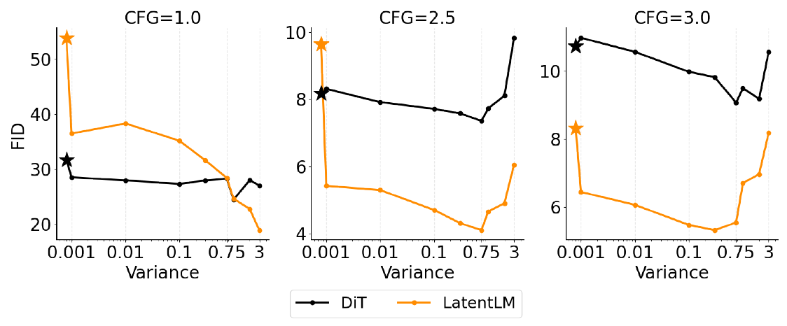
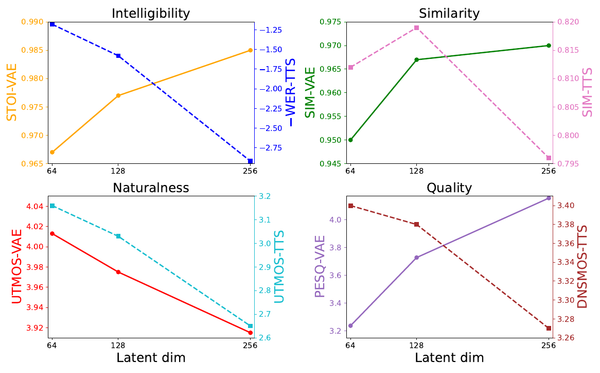
Source: LatentLM paper, Figure 6, p. 8. What to see: in the left panel (no classifier-free guidance) the orange LatentLM curve improves as tokenizer variance grows while the black DiT curve stays nearly flat; in the center and right panels, guidance bends the LatentLM curves into a U whose high-variance arm rises again. In every panel the star markers, tokenizers tuned for image-level latent diffusion with tiny variance, sit far above the LatentLM curve and roughly on the DiT curve.
LatentLM trains image tokenizers across a sweep of fixed variances and evaluates each latent space under two generators: DiT, a non-autoregressive diffusion Transformer that denoises all positions jointly and so never feeds a sampled latent back as conditioning context for later positions, and LatentLM, which does exactly that at every position. FID (Frechet Inception Distance, an image-generation quality score, lower is better) is nearly insensitive to tokenizer variance for DiT but, without classifier-free guidance (CFG, a sampling-time knob that amplifies conditioning), improves monotonically with variance for LatentLM. The small-variance tokenizers that serve image-level diffusion perfectly are the worst latent spaces for autoregressive consumption. The two generators differ in architecture and objective wholesale, so this is directional evidence rather than a single-variable ablation, but the variance sensitivity tracks exactly the presence of cross-position feedback. The U-shaped curves under guidance are the budget side of the knob: past the optimum, variance spent on robustness is capacity taken from the code. The sweep is image-domain with fixed rather than sampled variances; nothing isolates the knob for speech.
GIVT reports the same trade through a different knob. Raising the VAE's KL weight makes reconstruction worse but autoregressive sampling better, and since reconstruction quality is a ceiling generation cannot exceed, the knob trades ceiling height for how closely the generator approaches it. This is the same decoupling between reconstruction and generation usability documented for non-autoregressive generators in SAME Makes Generation Difficulty an Autoencoder Training Loss. How to budget the trade across KL targets, noise injection, normalization, and decoder tolerance is the subject of Latent Audio Encoders: Reconstruction Sets the Ceiling, Not the Ranking, which treats latent regularization as deciding which component absorbs prediction error.
VibeVoice is the production endorsement. Its frozen acoustic tokenizer is a sigma-VAE using the sampled-sigma scheme with C_sigma = 0.5, adopted, in the paper's words, to mitigate variance collapse in autoregressive modeling settings, and the system generates up to 90 minutes of multi-speaker audio, the regime where dense latent drift has the longest lever arm. That working value is the only published speech-side variance datapoint we know of in this family; treat it as a starting point, not a tuned optimum.
Diffusion samplers have the same mismatch, and the same fix works
The exposure-bias template is not specific to autoregression over positions; it applies wherever a model consumes self-generated state. A diffusion sampler is the clearest second instance: training denoises ground-truth noised inputs, but at inference each denoising step receives the previous step's prediction, a mismatch Ning et al. describe as the exposure bias problem shared with autoregressive methods, with prediction errors accumulating along the chain. Their fix is the sigma-VAE move at the sampler level: perturb the training input with extra Gaussian noise to simulate inference-time prediction error, leaving the target untouched. The perturbation is semantics-free, so the original target remains a valid answer for the perturbed input (the same property that makes the noisy posterior sample a correct training pair above), and the retrained ADM-IP model matches its baseline's quality with far fewer sampling steps (80 versus 1,000 in their headline comparison). Wherever a model consumes self-generated state, this is the property to check first: the supervision attached to a corrupted or self-generated context must still be correct for that context.
Sources
- Ranzato et al., 2016, Sequence Level Training with Recurrent Neural Networks (arXiv:1511.06732): naming and definition of exposure bias (intro and teacher forcing section); the misaligned-target example against data-as-demonstrator (scheduled sampling section); MIXER mechanism and results (sequence-level training section).
- Bengio et al., 2015, Scheduled Sampling for Sequence Prediction with Recurrent Neural Networks (arXiv:1506.03099): error-amplification framing (teacher forcing section); the sampling mechanism, decay schedules, no-backprop detail, task results, and the always-sampling failure (scheduled sampling section).
- Huszar, 2015, How (not) to Train your Generative Model: Scheduled Sampling, Likelihood, Adversary? (arXiv:1511.05101): improperness of the scheduled sampling objective, the product-of-marginals optimum, and the prefix-ignoring optimal model (scheduled sampling section).
- Ross, Gordon, Bagnell, 2011, A Reduction of Imitation Learning and Structured Prediction to No-Regret Online Learning (arXiv:1011.0686): quadratic-versus-linear compounding bounds, Theorems 2.1 and 3.2, and the DAgger mechanism (teacher forcing and sequence-level training sections).
- Arora et al., 2022, Why Exposure Bias Matters: An Imitation Learning Perspective of Error Accumulation in Language Generation (arXiv:2204.01171): measured error accumulation and perplexity's blindness to it (teacher forcing section).
- He et al., 2021, Exposure Bias versus Self-Recovery: Are Distortions Really Incremental for Autoregressive Text Generation? (arXiv:1905.10617): the self-recovery finding bounding in-domain damage (model-error section).
- Wang and Sennrich, 2020, On Exposure Bias, Hallucination and Domain Shift in Neural Machine Translation (arXiv:2005.03642): in-domain versus out-of-domain hallucination rates and the minimum risk training result (model-error section).
- Sabour, Chan, Norouzi, 2018, Optimal Completion Distillation for Sequence Learning (arXiv:1810.01398): edit-distance-optimal target relabeling on model-sampled prefixes (sequence-level training section).
- Lamb et al., 2016, Professor Forcing: A New Algorithm for Training Recurrent Networks (arXiv:1610.09038): adversarial matching of teacher-forced and free-running dynamics (sequence-level training section).
- Sun et al., 2024, Multimodal Latent Language Modeling with Next-Token Diffusion / LatentLM (arXiv:2412.08635): next-token diffusion definition (continuous-latent section); sigma-VAE formulation, Section 2.3; the variance sweep, Section 3.1.3 and Figure 6, p. 8 (variance shaping section, including the reproduced figure).
- Tschannen, Eastwood, Mentzer, 2023, GIVT: Generative Infinite-Vocabulary Transformers (arXiv:2312.02116): Gaussian-mixture head (continuous-latent section); the KL-weight versus sampling-quality trade and the reconstruction ceiling (variance shaping section).
- Li et al., 2024, Autoregressive Image Generation without Vector Quantization / MAR (arXiv:2406.11838): diffusion loss as the per-token distribution model for continuous tokens (continuous-latent section).
- VibeVoice: Expressive Podcast Generation with Next-Token Diffusion (OpenReview, ICLR 2026): sigma-VAE adoption rationale, Section 2.1; C_sigma = 0.5, Appendix F; 90-minute multi-speaker generation, abstract (variance shaping section). The arXiv technical report (arXiv:2508.19205) omits the appendix carrying the C_sigma value.
- Ning et al., 2023, Input Perturbation Reduces Exposure Bias in Diffusion Models (arXiv:2301.11706): the diffusion-sampler instance and the input-perturbation fix (final section).
Related Diffio Posts
- Latent Audio Encoders: Reconstruction Sets the Ceiling, Not the Ranking: the regularization-as-error-absorption framing this post's variance section builds on.
- SAME Makes Generation Difficulty an Autoencoder Training Loss: the reconstruction-versus-generation decoupling in a non-autoregressive setting.