
How To Train A Latent Audio Encoder
A latent audio encoder has a small-looking job.
audio -> encoder -> latent -> decoder -> audio
If the goal is compression, this sketch is almost enough. The encoder should make the middle object small, and the decoder should reconstruct the signal.
Most modern continuous audio encoders are trained for a harder loop.
audio -> encoder -> z

text, prompt, noisy audio, video, or context -> generator -> z_hat

z_hat -> decoder -> audio
The deployed decoder sees more than the encoder's clean latent. It sees a latent predicted by another model: an autoregressive Transformer, a diffusion head, a flow model, a bridge model, or a restoration model. That predicted latent will be slightly wrong.
This changes the training target. A useful latent audio encoder is not finished when D(E(x)) sounds good. It is finished when another model can predict, sample, edit, or condition on the latent, and the decoder can survive the errors that model makes.
That is the main design rule.
Train the interface, not just the codec.
The Interface Contract
The latent sequence is an API between systems. It has a clock, a width, a coordinate system, a distribution, and a set of invariances.
z[t] means:
    a time slice?
    a text-token span?
    a chunk summary?
    a degraded-to-clean bridge state?
    a global style variable?
Those choices decide what the downstream model has to predict.
A 10 Hz sequence of 64-dimensional vectors is not equivalent to a 5 Hz sequence of 128-dimensional vectors, even if the scalar count per second is similar. The first asks the model to make more frequent local updates. The second asks each position to summarize a longer acoustic span.
This is why latent rate and width should be selected with the downstream model in the loop. LongCat-AudioDiT is a clean example: its Wav-VAE ablations show that higher-dimensional latents can improve reconstruction while hurting TTS generation under a fixed TTS budget. The paper also varies latent frame rate and finds that the best reconstruction setting and the best generation setting need not match.
Target-KL audio VAEs make the same point from a different direction. They train continuous audio VAEs at controlled KL targets so the latent bitrate becomes an experimental variable. The useful setting is not simply "more reconstruction." It is the compression level that the downstream diffusion model can predict.
SAME pushes the idea harder for music. It uses 4096x temporal compression and a 256-dimensional latent, then adds flow-matching, semantic, contrastive, and phase-aware pressures so the latent remains usable for generation at that high compression ratio.
The right first question is therefore not:
How good is the autoencoder?
It is:
What prediction problem did the autoencoder create?
Choose The Coordinate System First
Before picking a KL weight or a discriminator, choose what one latent position means.
| Latent topology | Typical use | What the downstream model must do |
|---|---|---|
| Uniform time grid | VIBEVOICE, CLEAR, LongCat, Stable Audio Open | Predict acoustic state at fixed time steps. |
| Text-token-aligned vectors | TADA | Predict one acoustic object per text token plus timing metadata. |
| Chunk summaries | Music2Latent2 | Predict or decode unordered summaries for longer audio chunks. |
| Degraded-to-clean latent states | VoiceBridge, LatentFlowSR | Map one latent domain into another. |
| Global or segment variables | VAE-Loop, older speech VAEs | Control style, expression, speaker, or segment-level structure. |
Uniform time latents are natural for waveform reconstruction and many diffusion or AR systems. Text-aligned latents make the speech sequence much shorter, but they force the encoder to solve an alignment problem. Chunk summaries help with long-form compression, but they make local editing and precise timing more complicated. Restoration latents may deliberately move degraded input toward a clean target, which makes them poor neutral codecs and useful task interfaces.
The topology choice should come before the loss list. Otherwise the training recipe can optimize the wrong object with great care.
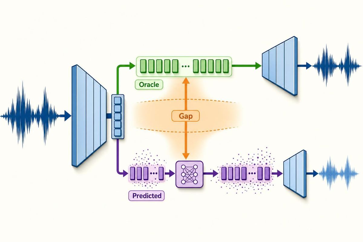
Build The Oracle, Then Break It
Start with the ordinary autoencoder path.
x -> E -> z -> D -> x_hat
This gives the oracle floor: how good the decoder can sound when the latent comes from the encoder. Use the usual audio infrastructure here: multi-resolution STFT or mel losses, adversarial losses, feature matching, and task-specific spectral terms such as CQT, complex STFT, mid/side stereo, phase-aware losses, or discriminator variants.
Then add the missing rows.
| Decode path | What it tests |
|---|---|
D(E(x)) |
Clean oracle reconstruction. |
D(sample(q(z|x))) |
Whether posterior sampling damages quality. |
D(E(x) + eps) |
Whether the decoder tolerates calibrated latent error. |
D(z_hat) |
Whether the downstream model's latents decode well. |
D(project(z_hat)) |
Whether failures come from off-manifold latents. |
This table is the predicted-latent gap. It is the difference between the clean oracle and the latent distribution the generator will actually emit.
Several papers are already moving in this direction. LatentFlowSR injects noise into the autoencoder latent during training so the decoder can handle latents predicted by its conditional-flow model. SAME adds latent noise and trains a small diffusion model that eventually backpropagates into the encoder. SALAD reports that sampled posterior targets work better than mean-only targets for its per-token latent diffusion setup. AudioLDM discusses the mismatch risk that comes from training the autoencoder and latent diffusion model as separate modules.
The practical version is simple: keep a small downstream probe alive during encoder training. It can be much smaller than the final generator. Cache:
mu
sample(q)
E(x) + calibrated_noise
z_hat from a probe predictor
Then decode all four. A checkpoint that wins on D(E(x)) but loses badly on D(z_hat) is a codec checkpoint, not a generation checkpoint.
Regularization Is Error Ownership
KL, fixed variance, target-KL, soft normalization, tanh bounds, latent dropout, variance floors, and latent noise all answer the same engineering question:
Who absorbs prediction error?
One choice pushes the latent toward a simple prior so the predictor has an easier job. Another lets the latent stay sharp and forces the predictor to learn a harder distribution. Another trains the decoder to accept imperfect latents.
These are not aesthetic VAE choices. They assign responsibility.
Target-KL makes this visible by setting a desired KL and sweeping the rate. Under-regularized latents can reconstruct well while creating a difficult diffusion target. Over-regularized latents can be easy to predict and still cap audio quality. The interesting operating point is the middle of that rate-distortion curve for the downstream model.
LatentFlowSR chooses decoder tolerance directly by adding latent noise. KALL-E uses a Flow-VAE so the AR model predicts the next latent distribution rather than a point. VIBEVOICE, LatentLM, and SemaVoice use sigma-VAE style choices to make low-rate continuous speech latents workable for autoregressive prediction. SAME uses soft-normalization and auxiliary generation pressure rather than a standard VAE bottleneck.
A useful validation dashboard should split the regularization term by place instead of stopping at an average:
per-channel mean and std
latent norm distribution
KL per second
outlier rate
posterior sample vs mean decode delta
silence vs transients
speech vs music vs effects
clean vs reverberant or noisy examples
predicted-latent residuals
Average KL can look healthy while one channel or one acoustic regime carries the debt.
Semantic Teachers Are Invariance Contracts
Many newer systems add a teacher: WavLM, HuBERT, Whisper, CLAP, CTC alignment, chroma regression, interaural-level-difference regression, or contrastive audio-text losses.
The tempting description is "semantic alignment." The more useful description is an invariance contract.
The teacher declares which differences the latent may collapse and which differences must remain measurable.
| Factor | Should it survive in z? |
Typical probe |
|---|---|---|
| Spoken content | Usually yes for TTS | ASR/WER, CTC, phoneme probes |
| Speaker identity | Often yes for voice cloning | speaker verification, SIM |
| Room or microphone color | Product-dependent | channel classifier, prompt-match metric |
| Prosody and rhythm | Usually yes | F0, energy, duration, rhythm probes |
| Stereo position | Yes for music/general audio | ILD, mid/side, spatial metrics |
| Background noise or degradation | Depends on task | restoration target and leakage probe |
VIBEVOICE shows the tradeoff clearly. Its coupled tokenizer improves content relative to an acoustic-only path, but speaker similarity drops hard. The final hybrid design keeps acoustic and semantic paths separate so the system can improve intelligibility without making one narrow latent carry every job.
Semantic-VAE adds WavLM-style alignment to a speech VAE and reports better TTS performance while preserving reconstruction quality. Its ablations also show that the choice of SSL layer and alignment loss matters. SALAD-VAE uses CLAP distillation and contrastive learning for semantic audio compression. SAME uses music-specific regressions and contrastive alignment, including chroma and stereo-related signals.
The builder move is to write a retain/collapse ledger before training:
retain:
    words
    speaker
    prosody
    pitch
    stereo image

collapse or normalize:
    background hiss?
    room tone?
    loudness?
    recording format?
The question marks matter. A podcast voice-cloning model may need room tone because prompt atmosphere affects perceived identity. A restoration model may need to remove it. A music generator may need stereo geometry. A speech understanding tokenizer may want to discard it.
The same teacher loss can be a feature in one system and a bug in another.
Stage Training By Gradient Ownership
A single blended loss can hide a conflict.
reconstruction wants: waveform detail
semantic teacher wants: content structure
prior shaping wants: predictable latents
decoder polish wants: perceptual texture
If all of those gradients hit the encoder forever, the latent can drift in ways that are hard to diagnose. Several systems stage the work instead.
RAVE learns the representation first, then freezes the encoder while improving the decoder adversarially. Stable Audio Open and long-form music VAEs use decoder fine-tuning stages. SAME uses warmup before letting diffusion and contrastive losses shape the encoder. TADA and VoiceBridge separate encoder formation, decoder adaptation, and task-specific latent modeling.
A practical schedule looks like this:
phase 1: reconstruction + light prior shaping
phase 2: semantic or task pressure, with protected-factor probes
phase 3: frozen-encoder decoder polish
phase 4: predicted-latent replay calibration
phase 5: short joint tune, only if latent drift stays controlled
At each boundary, log which objective owns the encoder:
encoder gradient norm by loss
latent norm and KL drift
teacher alignment score
oracle reconstruction
predicted-latent decode quality
speaker/content/channel/prosody probes
This turns staging from folklore into a debugging tool.
Task-Shaped Encoders Need Two Oracles
Some continuous audio encoders should be bad neutral codecs.
AUTOVC narrows a bottleneck to remove source-speaker information. TADA aligns audio to text tokens. VoiceBridge maps degraded speech toward clean latent targets. LatentFlowSR trains for super-resolution in latent space. Semantic-VAE optimizes a representation for TTS learnability.
If those systems are judged only by clean audio -> encoder -> decoder -> clean audio, the evaluation can reward leakage and punish the intended task.
Use two oracle floors:
| Oracle | Path | What it answers |
|---|---|---|
| Neutral oracle | clean x -> E -> D -> x |
How much audio can the codec preserve? |
| Task oracle | task input -> E_task -> D/task head -> target |
Did the latent keep the right evidence for the task? |
For restoration, the task oracle may start from degraded audio and target clean audio. For voice conversion, it may target content preservation with speaker identity moved outside the bottleneck. For text-aligned TTS, it may measure whether the acoustic vector follows the text token and duration contract.
The leakage probes should match the contract:
content leakage
speaker leakage
channel leakage
degradation leakage
prosody leakage
event leakage
Without those probes, a task-shaped encoder can look worse for the exact reason it works.
A Training Checklist
Here is the practical recipe I would start from.
- Define the downstream model before the encoder. Decide whether the latent will be predicted by AR, diffusion, flow, restoration, editing, or control.
- Choose latent topology before latent rate. Pick uniform time, text-aligned, chunk summary, bridge-state, segment, or global coordinates.
- Sweep rate and width with the downstream budget fixed. Keep the generator size, data, and decoding policy stable. Compare both oracle reconstruction and predicted-latent output.
- Train the reconstruction floor. Use the right audio losses for the domain: MR-STFT, mel, CQT, complex STFT, phase, stereo, adversarial, and feature matching as needed.
- Add prior shaping as an error-ownership decision. Use KL, target-KL, sigma-VAE variance, soft bounds, dropout, or noise because a specific predictor or decoder needs it.
- Add semantic teachers with a retain/collapse ledger. Protect speaker, prosody, channel, stereo, pitch, or degradation factors when the product needs them.
- Keep a predicted-latent probe during training. Decode
E(x), samples, noised latents, andz_hatfrom a small predictor. Checkpoint on the gap as well as the oracle. - Stage by gradient ownership. Freeze the encoder for decoder polish when the latent geometry is already useful. Re-open joint training only when drift is measured.
- Report dual oracles for task-shaped encoders. A restoration, conversion, text-aligned, or semantic encoder should be judged against its task contract as well as its neutral reconstruction floor.
Technical Takeaways
Add The Predicted-Latent Gap
The most important row in the evaluation table is the one most codec reports do not include:
D(E(x)) vs D(z_hat)
A continuous encoder can win oracle reconstruction while losing as a generation interface. The useful diagnostic is a side-by-side decode of clean latents, posterior samples, calibrated noised latents, and actual predicted latents.
Evidence comes from several directions: Target-KL shows that reconstruction and downstream diffusion quality can pull apart; LongCat shows that better Wav-VAE reconstruction can hurt fixed-budget TTS generation; LatentFlowSR trains decoder tolerance with latent noise; SAME lets downstream flow pressure shape the latent space.
The implementation consequence is concrete. Keep a small predictor or residual proxy in the encoder training loop, and gate checkpoints on the oracle-to-predicted gap.
Rate, Width, And Topology Define The Prediction Problem
Latent Hz is not just a compression number. Width is not just capacity. Topology is not just bookkeeping.
Together they define the object another model must predict. Equal scalar counts per second can create different failures because temporal frequency and channel width bundle acoustic evidence differently. Text-aligned vectors, chunk summaries, bridge latents, and uniform waveform grids are different coordinate systems.
The useful experiment is a fixed-generator sweep: vary rate, width, and topology while holding downstream model budget stable. Split failures into alignment drift, prosody drift, speaker/timbre loss, local editability, oracle reconstruction, and predicted-latent quality.
Every Training Pressure Should Declare Ownership
KL, semantic teachers, augmentations, dropout, latent noise, decoder freezing, and adversarial polish should each say what they own.
KL / target-KL: prior difficulty
latent noise: decoder tolerance
semantic teacher: content or text alignment
augmentation: invariance choice
frozen decoder polish: waveform texture without moving the latent
When a loss cannot declare its job, it becomes hard to debug. When it can, the encoder training run has clear phase boundaries, clear probes, and clear failure ownership.
Sources
- Taming Audio VAEs via Target-KL Regularization
- LongCat-AudioDiT: High-Fidelity Diffusion Text-to-Speech in the Waveform Latent Space
- SAME: A Semantically-Aligned Music Autoencoder
- LatentFlowSR: High-Fidelity Audio Super-Resolution via Noise-Robust Latent Flow Matching
- VoiceBridge: General Speech Restoration with One-step Latent Bridge Models
- Semantic-VAE: Semantic-Alignment Latent Representation for Better Speech Synthesis
- VibeVoice Technical Report
- CLEAR: Continuous Latent Autoregressive Modeling for High-quality and Low-latency Speech Synthesis
- TADA: A Generative Framework for Speech Modeling via Text-Acoustic Dual Alignment
- SALAD-VAE: Semantic Audio Compression with Language-Audio Distillation
- Music2Latent2: Audio Compression with Summary Embeddings and Autoregressive Decoding
- Stable Audio Open
- RAVE: A variational autoencoder for fast and high-quality neural audio synthesis
- KALL-E: Autoregressive Speech Synthesis with Next-Distribution Prediction


