VibeVoice: Frame Rate Is the Context Budget for Long-Form TTS
VibeVoice is Microsoft Research's open-weights system for zero-shot, multi-speaker, long-form speech synthesis: give it a short voice sample per speaker and a script, and a Qwen2.5 backbone generates podcast-style conversation, turn-taking and breaths included, in one streaming left-to-right pass.
VibeVoice is Microsoft Research's open-weights system for zero-shot, multi-speaker, long-form speech synthesis: give it a short voice sample per speaker and a script, and a Qwen2.5 backbone generates podcast-style conversation, turn-taking and breaths included, in one streaming left-to-right pass. In our map of the modern TTS stack it sits in the continuous-latent autoregressive family. The abstract claims up to 90 minutes of audio with up to 4 speakers; the quantitative evaluation stops at 30 minutes, and the paper never reconciles the two figures. Podcast generation itself is table stakes (NotebookLM, MoonCast, and FireredTTS2 all ship it).
The load-bearing choice is the speech tokenizer's frame rate: 7.5 frames per second, a 3200x downsampling of the 24 kHz waveform, far below the discrete codecs in the paper's comparison tables (40 to 600 tokens per second). That one rate is what fits a 90-minute conversation into a language model's context window. Everything distinctive downstream exists to make the rate survivable: the latent widens to 64 continuous dimensions, a diffusion head replaces the softmax, and semantic content gets its own encoder.
A 7.5 Hz tokenizer fits 90 minutes in context; the cost lands in channel width
The acoustic tokenizer emits one 64-dimensional continuous latent per 133 ms of audio, so 90 minutes of speech is 40,500 positions: inside the 65,536-token training context (the final phase of a length curriculum that starts at 4,096) with room left for the script. Long-form generation is then dense attention over one flat sequence, with no chunking, sliding windows, or hierarchical outline model.
What compression removes from the time axis has to reappear in the channel dimension if reconstruction quality is to hold, so the latent must widen as the rate falls. LatentLM, the paper VibeVoice takes its tokenizer recipe from, measures the conversion directly, and the compensation has a ceiling: its deepest compression setting degrades despite a wider latent. VibeVoice's 7.5 Hz / 64-dim operating point is the same one LatentLM ships for speech. SAME makes the same trade for music at 4096x, and our latent audio encoder post maps the general design space: rate, width, and latent geometry jointly define the prediction problem the downstream generator faces.
A 64-dim continuous channel is also what retires the softmax. A softmax head picks one codebook entry per step, and no practical codebook covers the information that survives 3200x compression. The discrete route shards each frame across a stack of residual vector quantization (RVQ) codebooks, each quantizing what the previous ones missed: MOSS-TTS, the strongest discrete system at comparable ambition, spends 32 codebooks on every 12.5 Hz frame and pays for them with an inner per-frame decoding loop. VibeVoice samples the whole 64-dim vector jointly through a diffusion head, paying an inner loop of denoising steps instead. A continuous head does not have to be a diffusion head (MELLE regresses mel frames with a variance-augmented head), but denoising from noise samples the full conditional distribution where a regression head commits to a parametric family.
What 7.5 Hz costs in reconstruction:
| Tokenizer | Tokens/s | PESQ | STOI | UTMOS |
|---|---|---|---|---|
| Encodec (8 codebooks) | 600 | 2.72 | 0.939 | 3.04 |
| DAC (4 codebooks) | 400 | 2.74 | 0.928 | 3.43 |
| WavTokenizer | 75 | 2.37 | 0.914 | 4.05 |
| VibeVoice acoustic | 7.5 | 3.07 | 0.828 | 4.18 |
LibriTTS test-clean, from the paper's Table 3. PESQ is an intrusive perceptual speech-quality score with a 4.5 ceiling, STOI a 0–1 intelligibility score computed against the reference, UTMOS a learned 1–5 predictor of human quality ratings.
The continuous tokenizer leads PESQ and UTMOS at one tenth of WavTokenizer's token rate, but token rate is a sequence-length unit, not an information unit: at 16-bit floats the 64-dim latent stream is roughly 7.7 kbps, above every discrete row in the table. The win is positions in the LM's context, not bitrate efficiency.
The weak column is STOI, which the authors attribute to training on podcast audio that deliberately skipped noise reduction. LibriTTS test-clean is clean, so the mismatch runs through the decoder's learned prior: at 3200x the decoder synthesizes fine detail rather than copying it, and detail synthesized under a noisy-podcast prior diverges from the clean reference at exactly the short-time envelope level STOI compares.
The sigma-VAE tokenizer sets latent variance for the generator that consumes it
The tokenizer is a mirror-symmetric encoder-decoder pair, roughly 340M parameters each, built from seven stages of Transformer blocks whose self-attention is replaced by 1D depth-wise causal convolutions, so encoding and decoding stream; training follows DAC's adversarial recipe. The paper calls it a tokenizer, but it is a VAE variant from LatentLM, the same paper that supplies the generation recipe: the encoder predicts only a mean, and the latent is
z = mu + sigma * epsilon, epsilon ~ N(0,1), sigma ~ N(0, C_sigma)
with sigma a scalar shared across all 64 channels, drawn fresh per example; VibeVoice sets C_sigma = 0.5.
Taking variance away from the encoder makes the latent space's noise floor a design parameter instead of a training outcome. A vanilla VAE under reconstruction pressure lets per-channel variances collapse toward zero, and once they collapse, every property the generator depends on, the scale of the latents, the spacing between codes, the smoothness of the distribution the diffusion head must learn to sample, is whatever reconstruction happened to leave behind. Fixing sigma pins those properties: information must be carried by mean displacements large enough to clear a noise band of known, channel-uniform width. LatentLM tuned the knob against the consumer rather than the reconstruction: across a sweep of tokenizer variances, generation quality for a next-token-diffusion model tracks the variance while an image-level diffusion model over the same latents is indifferent to it. The band is also the system's tolerance to its own sampling error: every generated latent re-enters the context, and an error smaller than the trained band lands inside the distribution the decoder and the LM already know. Exposure bias, and how variance shaping buys margin against it, gets a full treatment in its own post.
A diffusion head replaces the softmax; the backbone stays a standard autoregressive decoder
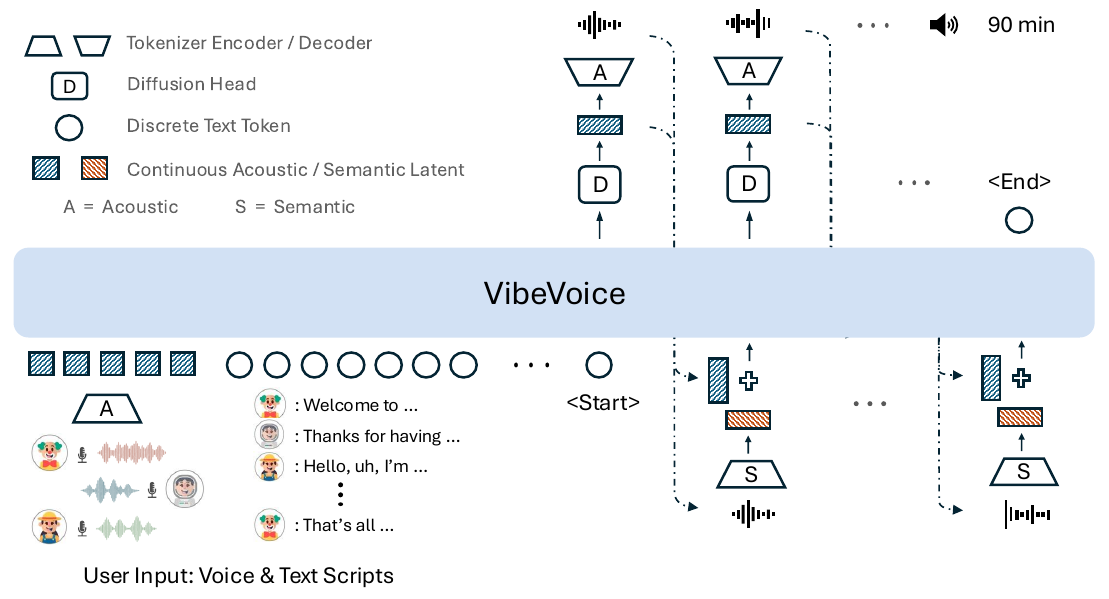
The prompt sequence concatenates, per speaker, an identifier and that speaker's voice-prompt latents (encoded by the acoustic encoder only; the script never includes the prompt's transcript), followed by speaker-tagged script text and a start-of-speech token. From there the backbone runs the standard autoregressive decoding loop with one substitution. At each step its hidden state conditions a diffusion head, 4 layers and roughly 123M parameters in the 1.5B configuration, in the style MAR introduced for image generation: trained with the standard DDPM noise-prediction L2 objective, it denoises Gaussian noise into the next acoustic latent while the backbone separately predicts whether to emit a termination token. The paper calls each step's output a speech segment without stating whether that is one 7.5 Hz frame or a packed group of frames, the report's largest reproduction gap.

VibeVoice paper, Figure 1, p. 2. Follow the right-hand loop: the diffusion head (D) emits an acoustic latent, the acoustic decoder (A) renders audio, and the semantic encoder (S) re-encodes that audio and adds it back into the next step's input.
At inference the head applies classifier-free guidance, extrapolating away from an unconditional prediction (derived here from the start-of-speech token's hidden state) to sharpen conditioning, at scale 1.3 with 10 denoising steps under DPM-Solver++, a fast ODE solver for diffusion sampling.
The cost structure keeps the language-model serving contract. The backbone runs autoregressively with a KV cache and dominates per-step latency at every profiled setting; the diffusion head's cost scales linearly with its step count, and the feedback path described next adds an acoustic decode and a semantic re-encode inside the loop at around 15 ms each. With everything included, the real-time factor (synthesis time over audio duration; below 1.0 is faster than real time) stays between 0.62 and 0.97 on a single A6000 across both model sizes, generating strictly left-to-right.
Semantic content comes from a second frozen encoder and feeds back as input, never as a generation target
The second tokenizer mirrors the acoustic encoder's architecture without the VAE machinery and is trained on an automatic speech recognition (ASR) proxy task: Transformer decoder layers learn to predict transcripts from its output, then the decoder is thrown away and the encoder is frozen. VibeVoice never generates semantic features. Instead, after the model produces a speech segment and decodes it to waveform, the history entry for that step combines two views of the same audio:
z_p,i = W_a * z_a,i + W_s * SemanticEnc(y_i)
where z_a is the generated acoustic latent, y is the rendered waveform, and z_p is the hybrid entry that actually enters the LLM's context, built from learned projections of both views.
The semantic entry is a deterministic function of the latent just produced, so it adds no new information to the context. What it adds is a representation: the phonetic content of that latent made explicit, where the acoustic latent buries it in texture optimized for reconstruction. The feedback closes a loop in which the LLM hears the phonetic content of its own output, so when generated audio drifts from the script, the drift is visible in the context rather than something the backbone must learn to extract. The loop is only closed at inference; during training the feedback path reads ground-truth audio, so any corrective use of it is learned implicitly.
That speech generation wants two representations is established lineage: AudioLM generated semantic tokens before acoustic ones, and SpeechTokenizer and Mimi distill semantic content into the first RVQ level of a discrete codec. What VibeVoice's ablation localizes is what goes wrong at a single continuous bottleneck, tested at matched model size and context (1.5B, 16K):
| History representation | 1-speaker WER-W | 3-speaker WER-W | Overall WER-W | Overall SIM-O |
|---|---|---|---|---|
| Acoustic latents only | 1.06 | 13.74 | 6.22 | 0.68 |
| One coupled latent (recon + ASR losses) | 6.79 | 1.40 | 3.55 | 0.45 |
| Hybrid: acoustic + semantic feedback | 1.93 | 2.50 | 1.84 | 0.64 |
Short-set podcast generation (the benchmark's under-12-minute subset), paper's Table 5; the overall columns pool one to four speakers. WER-W is the word error rate of a Whisper transcription of the generated audio against the input script; because the training data was itself filtered by Whisper agreement, the paper cross-checks with a second ASR (WER-N), which preserves the ranking. SIM-O is the cosine similarity between speaker embeddings of the generated audio and the original reference recording, dominated by timbre, the spectral character that makes a voice recognizable.
The acoustic-only row says reconstruction-grade latents preserve timbre (SIM-O matches the best setting) but lose content anchoring exactly when dialogue structure appears: single-speaker error is excellent, and at three speakers it explodes by an order of magnitude.
The coupled row tests the obvious repair, one encoder trained with reconstruction and transcript losses on a single latent, and shows the two objectives competing for fixed capacity. Content stabilizes where dialogue had broken it, but single-speaker error gets worse and the voice goes: overall SIM-O collapses to 0.45, the lowest of all settings in the paper, with the coupled tokenizer's raw reconstruction falling alongside it (PESQ 1.92 against the dedicated acoustic encoder's 2.98 on LibriSpeech test-clean). A 64-dim latent at 3200x has no slack for both objectives, and hard transcript-decoding pressure displaces exactly the texture that makes a voice identifiable. The shipped fix is more capacity, split by objective: a second full encoder, so reconstruction and transcript pressure never compete in one bottleneck.
The dilemma is narrower than the table makes it look. The hybrid pays a visible tax (worse single-speaker error and similarity than acoustic-only), and it binds only because VibeVoice keeps acoustic latents in the LM's context at all: cascades in the CosyVoice style dodge it by generating semantic tokens alone and restoring timbre in a reference-conditioned acoustic decoder, at the price of a second generation stage. SemaVoice serves both objectives with a single latent by softening the pressure, a cosine alignment to frozen WavLM features (a self-supervised speech encoder) at 15 Hz rather than transcript decoding at 7.5 Hz. And the ablation never tests other vehicles for semantic pressure, feeding back ASR text among them, so a separate frozen encoder is the tested fix, not the proven requirement.
Enhancement-free training data and few denoising steps protect the same signal: recording texture
The training corpus is roughly 80B tokens of internal pseudo-labeled podcast audio (the paper does not say how the count splits between text and audio frames), labeled by a pipeline of standard parts: voice-activity segmentation, Whisper transcription, diarization (assigning each segment to a speaker) via WeSpeaker embeddings and HDBSCAN clustering, then filtering by cross-ASR disagreement. The pipeline's one deliberate omission is speech enhancement: denoising removes interjections and prosodic cues along with the noise, so the tokenizer and the LM train on audio with its noise floor, reverb, and mouth sounds intact.
The same trade reappears at inference. The paper's Appendix J frames the diffusion head as a progressive denoiser: more solver steps refine detail but bias the output toward an idealized clean-speech distribution. The step/guidance sweep shows the two metrics pulling in opposite directions: word error is best near 10 steps, while SIM-O is highest at 5 steps and declines monotonically as steps increase.
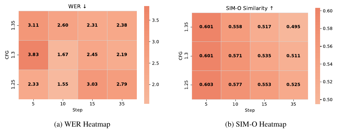
VibeVoice paper, Figure 3, p. 8. The global WER minimum (left) sits at 10 steps, while SIM-O (right) is highest in the 5-step column at every guidance scale and falls as steps grow.
The Appendix J spectrograms show what the extra steps remove: at 50 steps the model strips the prompt's environmental texture (room reverb, noise floor, microphone character), producing audio that is technically cleaner but spectrally mismatched from the reference the speaker embedding is computed on. A speaker's measured identity includes their recording environment, and over-denoising deletes evidence the metric expects to find. How much of that loss is perceptual rather than metric artifact is open: SIM-O is timbre-centric, and in an earlier round of the paper's human evaluation CosyVoice2 outscored VibeVoice-1.5B on SIM-O (0.68 vs 0.55) while human raters judged VibeVoice more similar to the prompt.
Results on VIBEVOICE-Eval and a 24-listener study: the 7B model leads, on an internal benchmark
Both evaluations are internal, so the podcast results locate the system rather than certify it: VIBEVOICE-Eval is 108 podcast samples (1 to 30 minutes, built with the same annotation pipeline from sources held out of training), and the listener study covers eight LLM-written two-speaker dialogues averaging 7.3 minutes, rated by 24 annotators.
| Model | Subjective avg (1–5) | WER-W | SIM-O |
|---|---|---|---|
| ElevenLabs v3 alpha | 3.40 | 2.39 | 0.623 |
| Gemini 2.5 Pro preview TTS | 3.66 | 1.73 | n/a |
| VibeVoice-1.5B | 3.54 | 1.11 | 0.548 |
| VibeVoice-7B | 3.76 | 1.29 | 0.692 |
Paper's Table 1; the subjective average pools realism, richness, and preference scores from the listener study. The paper reports no SIM-O for Gemini.
Scale buys consistency: the 7B leads every subjective dimension and posts the best speaker similarity, while the 1.5B keeps the lowest word error. On the long subset (12 to 30 minutes) the 7B holds WER-W 1.24 with SIM-O 0.75, where MoonCast, limited to two speakers and about ten minutes, crashes on long and 3-plus-speaker cases. Nothing past 30 minutes is measured, and the 7B never trained at the 65,536-token context phase (dropped for resource limits), so the 90-minute figure rests on the 1.5B's final training phase and the context arithmetic. Short-utterance generalization transfers: on the SEED benchmark's Chinese set the 1.5B stays competitive (character error rate 1.16) against systems running 25 to 50 Hz frame rates.
Sources
- VibeVoice: Expressive Podcast Generation with Next-Token Diffusion (OpenReview, ICLR 2026): architecture and training setup (Sections 2–3, Appendix F), reconstruction comparison (Table 3, Table 7), tokenizer ablations (Table 5, Appendices B and D), inference sweep and spectrograms (Figure 3, Appendix J), evaluation (Tables 1–2, Appendices G–I), inference cost (Table 8, Appendix E). Figures 1 and 3 reproduced from this paper. The shorter arXiv technical report (2508.19205) omits the appendices and ablation tables cited here.
- microsoft/VibeVoice on GitHub: released code and checkpoints.
- Multimodal Latent Language Modeling with Next-Token Diffusion (LatentLM, arXiv 2412.08635): sigma-VAE construction (Section 2.3), the tokenizer-variance sweep against DiT (Figure 6), compression-vs-width ablation (Table 6) cited in the frame-rate section.
- SemaVoice: Semantic-Aware Continuous Autoregressive Speech Synthesis (arXiv 2605.16964): the single-latent counterpoint cited in the tokenizer-split section.
Related Diffio Posts
- Exposure bias: why models trained on ground-truth history are brittle to their own samples, and how latent variance shaping buys margin.
- Classifier-free guidance: the conditioning-sharpening mechanism the diffusion head uses at inference.
- Latent Audio Encoders: Reconstruction Sets the Ceiling, Not the Ranking: the design space of continuous latents built for downstream generators.
- MOSS-TTS: Modeling The RVQ Stack: the discrete counterpoint, 32 codebooks per frame instead of one wide continuous latent.
- TTS Models: A Map Of The Modern Speech Stack: where the continuous-latent autoregressive family sits.
- SAME Makes Generation Difficulty an Autoencoder Training Loss: the same rate-for-width trade in music autoencoders.