MOSS-TTS Shows Local RVQ Conditioning Can Beat Delay Modeling

MOSS-TTS is a fully discrete text-to-speech system: text and prompt audio are serialized into language-model inputs, the model predicts audio codec tokens autoregressively, and a neural codec decoder turns those tokens back into waveform. In the Diffio map of modern TTS systems, that places it in the discrete codec-LM family, where the generated object is not a mel frame or a continuous latent but a matrix of codec tokens.
The MOSS comparison is internal: the report evaluates an 8B delay-pattern generator and a 1.7B Local Transformer under the same tokenizer and pretraining recipe. The comparison is not parameter matched, so it does not isolate causal RVQ depth from every local-module difference. It shows that in this released comparison, the smaller local architecture outperformed the larger delay backbone on the reported cloning metrics.
Low frame rate shifts modeling cost to RVQ depth
MOSS-Audio-Tokenizer makes long context possible by using a low frame rate and multiple RVQ layers per frame. It encodes 24 kHz audio at 12.5 frames per second.
Each frame contains 32 residual vector quantization (RVQ) layers. RVQ means the first codebook quantizes a coarse approximation, the next codebook quantizes what the first missed, and later codebooks keep refining the residual.
The report's final pretraining phase measures context in backbone time steps rather than scalar codec decisions. At 12.5 frame steps per second, its 64k-step training window covers about 85 minutes of audio before text, prompt tokens, and the delay model's 31-step edge overhead. The remaining modeling problem is the 32 ordered decisions attached to every frame.
The tokenizer can trade bitrate for residual depth because random quantizer dropout trains the decoder after randomly dropping later RVQ layers, so prefixes of the 32-layer stack remain valid codes. At this frame rate, each additional RVQ layer adds 125 bps.
| Bitrate | RVQ layers used | English/Chinese SIM | English/Chinese PESQ-WB |
|---|---|---|---|
| 1000 bps | 8 | 0.88 / 0.81 | 2.87 / 2.43 |
| 4000 bps | 32 | 0.97 / 0.93 | 3.69 / 3.30 |
MOSS-TTS Technical Report Table 2. SIM is cosine-scale speaker-embedding similarity; PESQ-WB is a wideband perceptual speech-quality score. These are tokenizer-oracle reconstruction rows, not a generator-factorization result.
The delay pattern preserves sequence length by interleaving RVQ layers
The delay pattern keeps the language-model sequence close to the audio frame count. Instead of flattening the RVQ stack into separate audio positions, it shifts each residual layer by its layer index. A T-frame utterance becomes T + 31 delayed backbone steps.
Each aligned step has one text/pad channel and one channel per RVQ layer. Channel 0 emits a normal text token on text-only steps and a dedicated pad symbol on audio-frame steps; the audio channels emit RVQ codes. Invalid delayed or padding positions are masked from the loss. In the delay model, one backbone hidden state feeds all channel heads.
This factorization is efficient for serving. The backbone is evaluated once per delayed step, and the output heads map the hidden state to token logits. This is why the report treats the delay architecture as the simpler route for long contexts, duration control, pronunciation control, and optimized inference backends.
The cost is that within-frame RVQ dependencies are represented across multiple delayed steps. Lower layers of a frame are emitted at earlier delayed steps than higher layers. By the time a higher layer is predicted, lower layers can influence it only through intervening input vectors, each built by adding codebook-specific embeddings from whatever delayed layers are present at that step. At any one delayed step, the audio heads are predicting channels from different original frames. The backbone is therefore not just modeling speech over time; it is also tracking incomplete RVQ code stacks across delayed positions.
The Local Transformer factorizes each frame autoregressively over RVQ layers
The Local Transformer keeps the frame aligned in time and adds a local autoregressive loop over channels. The temporal backbone produces one latent for the frame, then a lightweight local module predicts the text/pad channel and the RVQ layers in order. The text/pad channel keeps that stream in the same factorization as the audio layers. For audio frames it is the pad decision, followed by RVQ layers that condition on earlier layers from the same frame and on previous aligned steps.
That is the inductive bias the MOSS comparison supports for this residual stack. Later RVQ layers are not exchangeable labels; they are refinements of a residual left by earlier layers. Giving layer j the sampled lower-depth codes as direct context makes within-frame RVQ conditioning explicit. The delay pattern can represent that dependency only after the temporal backbone learns to route it through delayed positions.
Moshi is the immediate lineage for this choice: its RQ-Transformer predicts tokens bottom to top inside an audio step, and MOSS adapts that idea to the tokenizer's full RVQ stack. The tradeoff is steady-state cost. The local model runs an inner loop over channels, while the delay model cannot stream-decode a complete frame until the final RVQ layer arrives about 2.5 seconds later.
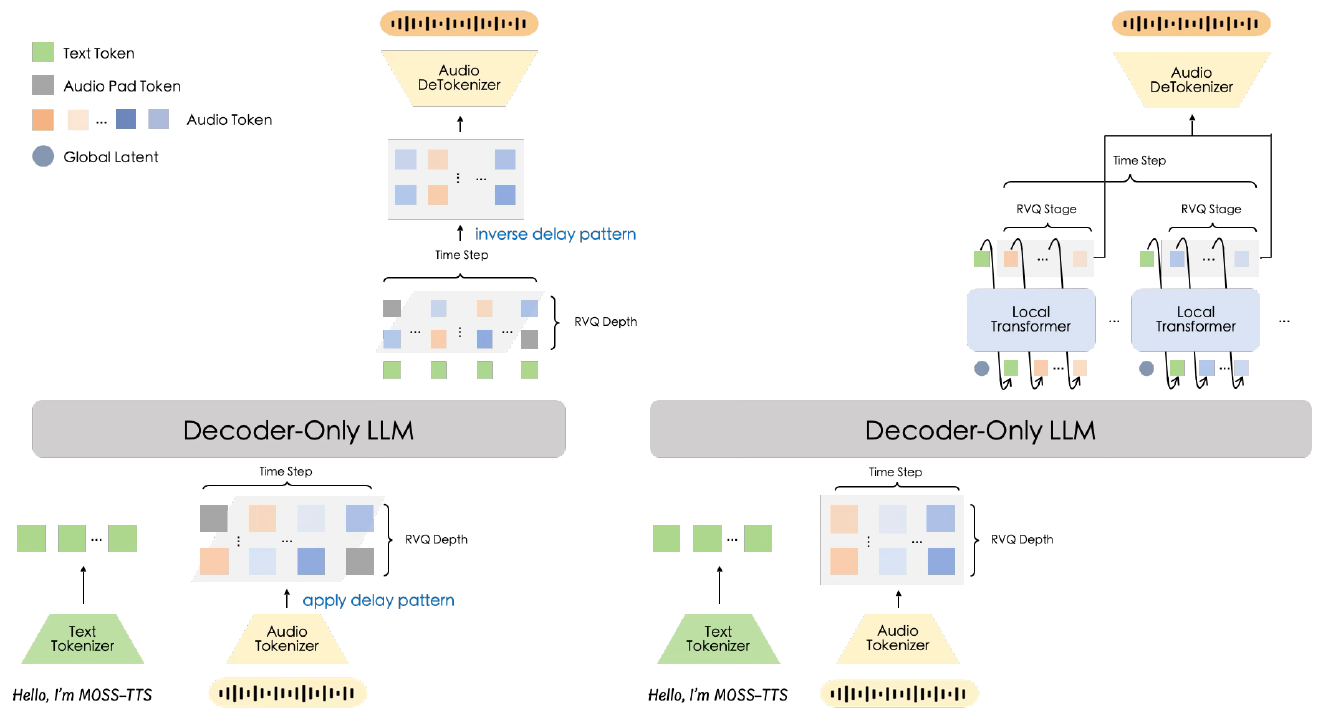
MOSS-TTS Technical Report, Figure 2, p. 8. Delay pattern on the left; frame-local autoregressive loop on the right.
The smaller local model wins the within-MOSS cloning comparison
Seed-TTS-eval reports WER for English word error rate, CER for Chinese character error rate, and SIM for speaker-embedding similarity on a percentage scale. This SIM scale differs from the 0-1 reconstruction SIM above.
| Model | Mode | Params | EN WER | EN SIM | ZH CER | ZH SIM |
|---|---|---|---|---|---|---|
| MOSS-TTS | Clone | 8B | 1.92 | 69.31 | 1.46 | 76.21 |
| MOSS-TTS-Local-Transformer | Clone | 1.7B | 1.87 | 71.74 | 1.33 | 77.24 |
| MOSS-TTS | Continuation | 8B | 1.84 | 70.86 | 1.37 | 76.98 |
| MOSS-TTS-Local-Transformer | Continuation | 1.7B | 1.93 | 73.28 | 1.44 | 79.62 |
Seed-TTS-eval, MOSS-TTS Technical Report Table 3. Lower WER/CER (%) is better; higher SIM (%) is better. The report gives no confidence intervals or listening-test variance for this table.
The Local Transformer outperforms the delay model in all four SIM cells, and the highest MOSS similarity value in the table is the local continuation model's Chinese SIM. In Clone mode it also lowers both content-error metrics. In Continuation mode the delay model has slightly lower WER/CER, but both models sit in the low-error regime where the report says manual review found many remaining mismatches to be ASR errors rather than audible pronunciation failures.
CV3-Eval extends the same direction to multilingual cloning, but only for content error. The Local Transformer has lower CER/WER than the delay model in every same-language comparison. Its average absolute improvement over the delay rows is about half a percentage point in both Clone and Continuation mode. That does not establish better speaker preservation outside English and Chinese, because CV3-Eval does not report speaker similarity, but it rules out the narrow explanation that the local model merely trades intelligibility for timbre.
The smaller model outperformed the larger one on the cloning cells the report uses to characterize the local-vs-delay tradeoff, so the evidence supports a scoped design claim: for this tokenizer and release, local conditioning over RVQ depth was the better cloning architecture.
Control and ultra-long results are delay-only
The control sections evaluate only the 8B delay model. Duration control, pronunciation control, and ultra-long generation are not reported for the Local Transformer.
The delay architecture supports the control and long-context experiments because it has a simpler single-backbone parameterization. For duration control, the prompt includes a requested audio-token count. The delay model's absolute relative duration error, the generated-duration miss divided by the requested duration, is 0.712% in Chinese and 0.723% in English, using paired pretraining examples with and without explicit token-count prompts rather than a separate duration-control fine-tune.
The ultra-long internal set separates content from speaker drift. In the English 50000+ input-character bucket, Clone WER reaches 17.49% and Continuation WER reaches 29.52%, while speaker similarity falls to 44.4% for Clone and 51.2% for Continuation.
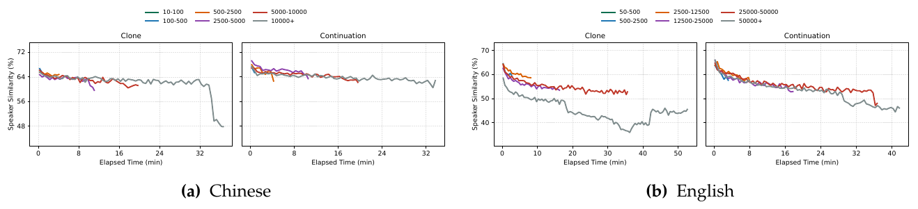
MOSS-TTS Technical Report, Figure 6, p. 21. The English longest-bucket curves separate early and remain low, showing that long-horizon degradation appears as cumulative speaker drift before every sample reaches a lexical failure.
Sources
- MOSS-TTS Technical Report: tokenizer geometry, Figure 2 architecture diagram, delay and Local Transformer objectives, Seed-TTS-eval Table 3, CV3-Eval Table 4, duration Table 5, ultra-long Table 6.
- MOSS-Audio-Tokenizer: CAT tokenizer motivation, end-to-end Transformer tokenizer context, and the tokenizer's role as a scalable audio-modeling interface.
- MusicGen: Simple and Controllable Music Generation: delay/interleaving-pattern lineage for multi-codebook audio-token modeling.
- Moshi: a speech-text foundation model for real-time dialogue: RQ-Transformer lineage and frame-local bottom-to-top token modeling.